Introduction
Miden VM is a zero-knowledge virtual machine written in Rust. For any program executed on Miden VM, a STARK-based proof of execution is automatically generated. This proof can then be used by anyone to verify that the program was executed correctly without the need for re-executing the program or even knowing the contents of the program.
Status and features
Miden VM is currently on release v0.14. In this release, most of the core features of the VM have been stabilized, and most of the STARK proof generation has been implemented. While we expect to keep making changes to the VM internals, the external interfaces should remain relatively stable, and we will do our best to minimize the amount of breaking changes going forward.
At this point, Miden VM is good enough for experimentation, and even for real-world applications, but it is not yet ready for production use. The codebase has not been audited and contains known and unknown bugs and security flaws.
Feature highlights
Miden VM is a fully-featured virtual machine. Despite being optimized for zero-knowledge proof generation, it provides all the features one would expect from a regular VM. To highlight a few:
- Flow control. Miden VM is Turing-complete and supports familiar flow control structures such as conditional statements and counter/condition-controlled loops. There are no restrictions on the maximum number of loop iterations or the depth of control flow logic.
- Procedures. Miden assembly programs can be broken into subroutines called procedures. This improves code modularity and helps reduce the size of Miden VM programs.
- Execution contexts. Miden VM program execution can span multiple isolated contexts, each with its own dedicated memory space. The contexts are separated into the root context and user contexts. The root context can be accessed from user contexts via customizable kernel calls.
- Memory. Miden VM supports read-write random-access memory. Procedures can reserve portions of global memory for easier management of local variables.
- u32 operations. Miden VM supports native operations with 32-bit unsigned integers. This includes basic arithmetic, comparison, and bitwise operations.
- Cryptographic operations. Miden assembly provides built-in instructions for computing hashes and verifying Merkle paths. These instructions use Rescue Prime Optimized hash function (which is the native hash function of the VM).
- External libraries. Miden VM supports compiling programs against pre-defined libraries. The VM ships with one such library: Miden
stdlibwhich adds support for such things as 64-bit unsigned integers. Developers can build other similar libraries to extend the VM's functionality in ways which fit their use cases. - Nondeterminism. Unlike traditional virtual machines, Miden VM supports nondeterministic programming. This means a prover may do additional work outside of the VM and then provide execution hints to the VM. These hints can be used to dramatically speed up certain types of computations, as well as to supply secret inputs to the VM.
- Customizable hosts. Miden VM can be instantiated with user-defined hosts. These hosts are used to supply external data to the VM during execution/proof generation (via nondeterministic inputs) and can connect the VM to arbitrary data sources (e.g., a database or RPC calls).
Planned features
In the coming months we plan to finalize the design of the VM and implement support for the following features:
- Recursive proofs. Miden VM will soon be able to verify a proof of its own execution. This will enable infinitely recursive proofs, an extremely useful tool for real-world applications.
- Better debugging. Miden VM will provide a better debugging experience including the ability to place breakpoints, better source mapping, and more complete program analysis info.
- Faulty execution. Miden VM will support generating proofs for programs with faulty execution (a notoriously complex task in ZK context). That is, it will be possible to prove that execution of some program resulted in an error.
Structure of this document
This document is meant to provide an in-depth description of Miden VM. It is organized as follows:
- In the introduction, we provide a high-level overview of Miden VM and describe how to run simple programs.
- In the user documentation section, we provide developer-focused documentation useful to those who want to develop on Miden VM or build compilers from higher-level languages to Miden assembly (the native language of Miden VM).
- In the design section, we provide in-depth descriptions of the VM's internals, including all AIR constraints for the proving system. We also provide the rationale for settling on specific design choices.
- Finally, in the background material section, we provide references to materials which could be useful for learning more about STARKs - the proving system behind Miden VM.
License
Licensed under the MIT license.
Miden VM overview
Miden VM is a stack machine. The base data type of the MV is a field element in a 64-bit prime field defined by modulus . This means that all values that the VM operates with are field elements in this field (i.e., values between and , both inclusive).
Miden VM consists of four high-level components as illustrated below.
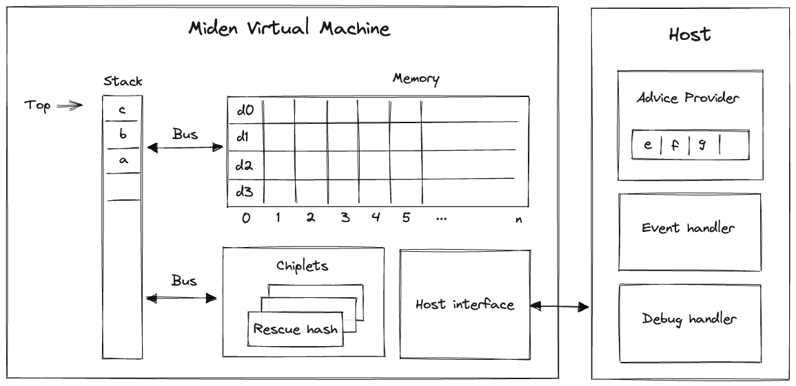
These components are:
- Stack which is a push-down stack where each item is a field element. Most assembly instructions operate with values located on the stack. The stack can grow up to items deep, however, only the top 16 items are directly accessible.
- Memory which is a linear random-access read-write memory. The memory is element-addressable, meaning, a single element is located at each address. However, there are instructions to read and write elements to/from memory both individually or in batches of four, since the latter is quite common. Memory addresses can be in the range .
- Chiplets which are specialized circuits for accelerating certain types of computations. These include Rescue Prime Optimized (RPO) hash function, 32-bit binary operations, and 16-bit range checks.
- Host which is a way for the prover to communicate with the VM during runtime. This includes responding to the VM's requests for non-deterministic inputs and handling messages sent by the VM (e.g., for debugging purposes). The requests for non-deterministic inputs are handled by the host's advice provider.
Miden VM comes with a default implementation of the host interface (with an in-memory advice provider). However, the users are able to provide their own implementations which can connect the VM to arbitrary data sources (e.g., a database or RPC calls) and define custom logic for handling events emitted by the VM.
Writing programs
Our goal is to make Miden VM an easy compilation target for high-level languages such as Rust, Move, Sway, and others. We believe it is important to let people write programs in the languages of their choice. However, compilers to help with this have not been developed yet. Thus, for now, the primary way to write programs for Miden VM is to use Miden assembly.
While writing programs in assembly is far from ideal, Miden assembly does make this task a little bit easier by supporting high-level flow control structures and named procedures.
Inputs and outputs
External inputs can be provided to Miden VM in two ways:
- Public inputs can be supplied to the VM by initializing the stack with desired values before a program starts executing. At most 16 values can be initialized in this way, so providing more than 16 values will cause an error.
- Secret (or nondeterministic) inputs can be supplied to the VM via the advice provider. There is no limit on how much data the advice provider can hold.
After a program finishes executing, the elements remaining on the stack become the outputs of the program. Notice that having more than 16 values on the stack at the end of execution will cause an error, so the values beyond the top 16 elements of the stack should be dropped. We've provided the truncate_stack utility procedure in the standard library for this purpose.
The number of public inputs and outputs of a program can be reduced by making use of the advice stack and Merkle trees. Just 4 elements are sufficient to represent a root of a Merkle tree, which can be expanded into an arbitrary number of values.
For example, if we wanted to provide a thousand public input values to the VM, we could put these values into a Merkle tree, initialize the stack with the root of this tree, initialize the advice provider with the tree itself, and then retrieve values from the tree during program execution using mtree_get instruction (described here).
Stack depth restrictions
For reasons explained here, the VM imposes the restriction that the stack depth cannot be smaller than . This has the following effects:
- When initializing a program with fewer than inputs, the VM will pad the stack with zeros to ensure the depth is at the beginning of execution.
- If an operation would result in the stack depth dropping below , the VM will insert a zero at the deep end of the stack to make sure the depth stays at .
Nondeterministic inputs
The advice provider component is responsible for supplying nondeterministic inputs to the VM. These inputs only need to be known to the prover (i.e., they do not need to be shared with the verifier).
The advice provider consists of three components:
- Advice stack which is a one-dimensional array of field elements. Being a stack, the VM can either push new elements onto the advice stack, or pop the elements from its top.
- Advice map which is a key-value map where keys are words and values are vectors of field elements. The VM can copy values from the advice map onto the advice stack as well as insert new values into the advice map (e.g., from a region of memory).
- Merkle store which contain structured data reducible to Merkle paths. Some examples of such structures are: Merkle tree, Sparse Merkle Tree, and a collection of Merkle paths. The VM can request Merkle paths from the Merkle store, as well as mutate it by updating or merging nodes contained in the store.
The prover initializes the advice provider prior to executing a program, and from that point on the advice provider is manipulated solely by executing operations on the VM.
Usage
Before you can use Miden VM, you'll need to make sure you have Rust installed. Miden VM v0.14 requires Rust version 1.85 or later.
Miden VM consists of several crates, each of which exposes a small set of functionality. The most notable of these crates are:
- miden-processor, which can be used to execute Miden VM programs.
- miden-prover, which can be used to execute Miden VM programs and generate proofs of their execution.
- miden-verifier, which can be used to verify proofs of program execution generated by Miden VM prover.
The above functionality is also exposed via the single miden-vm crate, which also provides a CLI interface for interacting with Miden VM.
CLI interface
Compiling Miden VM
To compile Miden VM into a binary, we have a Makefile with the following tasks:
make exec
This will place an optimized, multi-threaded miden executable into the ./target/optimized directory. It is equivalent to executing:
cargo build --profile optimized --features concurrent,executable
If you would like to enable single-threaded mode, you can compile Miden VM using the following command:
make exec-single
Controlling parallelism
Internally, Miden VM uses rayon for parallel computations. To control the number of threads used to generate a STARK proof, you can use RAYON_NUM_THREADS environment variable.
GPU acceleration
Miden VM proof generation can be accelerated via GPUs. Currently, GPU acceleration is enabled only on Apple Silicon hardware (via Metal). To compile Miden VM with Metal acceleration enabled, you can run the following command:
make exec-metal
Similar to make exec command, this will place the resulting miden executable into the ./target/optimized directory.
Currently, GPU acceleration is applicable only to recursive proofs which can be generated using the -r flag.
SIMD acceleration
Miden VM execution and proof generation can be accelerated via vectorized instructions. Currently, SIMD acceleration can be enabled on platforms supporting SVE and AVX2 instructions.
To compile Miden VM with AVX2 acceleration enabled, you can run the following command:
make exec-avx2
To compile Miden VM with SVE acceleration enabled, you can run the following command:
make exec-sve
This will place the resulting miden executable into the ./target/optimized directory.
Similar to Metal acceleration, SVE/AVX2 acceleration is currently applicable only to recursive proofs which can be generated using the -r flag.
Running Miden VM
Once the executable has been compiled, you can run Miden VM like so:
./target/optimized/miden [subcommand] [parameters]
Currently, Miden VM can be executed with the following subcommands:
run- this will execute a Miden assembly program and output the result, but will not generate a proof of execution.prove- this will execute a Miden assembly program, and will also generate a STARK proof of execution.verify- this will verify a previously generated proof of execution for a given program.compile- this will compile a Miden assembly program (i.e., build a program MAST) and outputs stats about the compilation process.debug- this will instantiate a Miden debugger against the specified Miden assembly program and inputs.analyze- this will run a Miden assembly program against specific inputs and will output stats about its execution.repl- this will initiate the Miden REPL tool.example- this will execute a Miden assembly example program, generate a STARK proof of execution and verify it. Currently, it is possible to runblake3andfibonacciexamples.
All of the above subcommands require various parameters to be provided. To get more detailed help on what is needed for a given subcommand, you can run the following:
./target/optimized/miden [subcommand] --help
For example:
./target/optimized/miden prove --help
To execute a program using the Miden VM there needs to be a .masm file containing the Miden Assembly code and a .inputs file containing the inputs.
Enabling logging
You can use MIDEN_LOG environment variable to control how much logging output the VM produces. For example:
MIDEN_LOG=trace ./target/optimized/miden [subcommand] [parameters]
If the level is not specified, warn level is set as default.
Enable Debugging features
You can use the run command with --debug parameter to enable debugging with the debug instruction such as debug.stack:
./target/optimized/miden run [path_to.masm] --debug
Inputs
As described here the Miden VM can consume public and secret inputs.
- Public inputs:
operand_stack- can be supplied to the VM to initialize the stack with the desired values before a program starts executing. If the number of provided input values is less than 16, the input stack will be padded with zeros to the length of 16. The maximum number of the stack inputs is limited by 16 values, providing more than 16 values will cause an error.
- Secret (or nondeterministic) inputs:
advice_stack- can be supplied to the VM. There is no limit on how much data the advice provider can hold. This is provided as a string array where each string entry represents a field element.advice_map- is supplied as a map of 64-character hex keys, each mapped to an array of numbers. The hex keys are interpreted as 4 field elements and the arrays of numbers are interpreted as arrays of field elements.merkle_store- the Merkle store is container that allows the user to definemerkle_tree,sparse_merkle_treeandpartial_merkle_treedata structures.merkle_tree- is supplied as an array of 64-character hex values where each value represents a leaf (4 elements) in the tree.sparse_merkle_tree- is supplied as an array of tuples of the form (number, 64-character hex string). The number represents the leaf index and the hex string represents the leaf value (4 elements).partial_merkle_tree- is supplied as an array of tuples of the form ((number, number), 64-character hex string). The internal tuple represents the leaf depth and index at this depth, and the hex string represents the leaf value (4 elements).
Check out the comparison example to see how secret inputs work.
After a program finishes executing, the elements that remain on the stack become the outputs of the program. Notice that the number of values on the operand stack at the end of the program execution can not be greater than 16, otherwise the program will return an error. The truncate_stack utility procedure from the standard library could be used to conveniently truncate the stack at the end of the program.
Fibonacci example
In the miden/masm-examples/fib directory, we provide a very simple Fibonacci calculator example. This example computes the 1001st term of the Fibonacci sequence. You can execute this example on Miden VM like so:
./target/optimized/miden run miden/masm-examples/fib/fib.masm
Capturing Output
This will run the example code to completion and will output the top element remaining on the stack.
If you want the output of the program in a file, you can use the --output or -o flag and specify the path to the output file. For example:
./target/optimized/miden run miden/masm-examples/fib/fib.masm -o fib.out
This will dump the output of the program into the fib.out file. The output file will contain the state of the stack at the end of the program execution.
Running with debug instruction enabled
Inside miden/masm-examples/fib/fib.masm, insert debug.stack instruction anywhere between begin and end. Then run:
./target/optimized/miden run miden/masm-examples/fib/fib.masm -n 1 --debug
You should see output similar to "Stack state before step ..."
Performance
The benchmarks below should be viewed only as a rough guide for expected future performance. The reasons for this are twofold:
- Not all constraints have been implemented yet, and we expect that there will be some slowdown once constraint evaluation is completed.
- Many optimizations have not been applied yet, and we expect that there will be some speedup once we dedicate some time to performance optimizations.
Overall, we don't expect the benchmarks to change significantly, but there will definitely be some deviation from the below numbers in the future.
A few general notes on performance:
- Execution time is dominated by proof generation time. In fact, the time needed to run the program is usually under 1% of the time needed to generate the proof.
- Proof verification time is really fast. In most cases it is under 1 ms, but sometimes gets as high as 2 ms or 3 ms.
- Proof generation process is dynamically adjustable. In general, there is a trade-off between execution time, proof size, and security level (i.e. for a given security level, we can reduce proof size by increasing execution time, up to a point).
- Both proof generation and proof verification times are greatly influenced by the hash function used in the STARK protocol. In the benchmarks below, we use BLAKE3, which is a really fast hash function.
Single-core prover performance
When executed on a single CPU core, the current version of Miden VM operates at around 20 - 25 KHz. In the benchmarks below, the VM executes a Fibonacci calculator program on Apple M1 Pro CPU in a single thread. The generated proofs have a target security level of 96 bits.
| VM cycles | Execution time | Proving time | RAM consumed | Proof size |
|---|---|---|---|---|
| 210 | 1 ms | 60 ms | 20 MB | 46 KB |
| 212 | 2 ms | 180 ms | 52 MB | 56 KB |
| 214 | 8 ms | 680 ms | 240 MB | 65 KB |
| 216 | 28 ms | 2.7 sec | 950 MB | 75 KB |
| 218 | 81 ms | 11.4 sec | 3.7 GB | 87 KB |
| 220 | 310 ms | 47.5 sec | 14 GB | 100 KB |
As can be seen from the above, proving time roughly doubles with every doubling in the number of cycles, but proof size grows much slower.
We can also generate proofs at a higher security level. The cost of doing so is roughly doubling of proving time and roughly 40% increase in proof size. In the benchmarks below, the same Fibonacci calculator program was executed on Apple M1 Pro CPU at 128-bit target security level:
| VM cycles | Execution time | Proving time | RAM consumed | Proof size |
|---|---|---|---|---|
| 210 | 1 ms | 120 ms | 30 MB | 61 KB |
| 212 | 2 ms | 460 ms | 106 MB | 77 KB |
| 214 | 8 ms | 1.4 sec | 500 MB | 90 KB |
| 216 | 27 ms | 4.9 sec | 2.0 GB | 103 KB |
| 218 | 81 ms | 20.1 sec | 8.0 GB | 121 KB |
| 220 | 310 ms | 90.3 sec | 20.0 GB | 138 KB |
Multi-core prover performance
STARK proof generation is massively parallelizable. Thus, by taking advantage of multiple CPU cores we can dramatically reduce proof generation time. For example, when executed on an 8-core CPU (Apple M1 Pro), the current version of Miden VM operates at around 100 KHz. And when executed on a 64-core CPU (Amazon Graviton 3), the VM operates at around 250 KHz.
In the benchmarks below, the VM executes the same Fibonacci calculator program for 220 cycles at 96-bit target security level:
| Machine | Execution time | Proving time | Execution % | Implied Frequency |
|---|---|---|---|---|
| Apple M1 Pro (16 threads) | 310 ms | 7.0 sec | 4.2% | 140 KHz |
| Apple M2 Max (16 threads) | 280 ms | 5.8 sec | 4.5% | 170 KHz |
| AMD Ryzen 9 5950X (16 threads) | 270 ms | 10.0 sec | 2.6% | 100 KHz |
| Amazon Graviton 3 (64 threads) | 330 ms | 3.6 sec | 8.5% | 265 KHz |
Recursive proofs
Proofs in the above benchmarks are generated using BLAKE3 hash function. While this hash function is very fast, it is not very efficient to execute in Miden VM. Thus, proofs generated using BLAKE3 are not well-suited for recursive proof verification. To support efficient recursive proofs, we need to use an arithmetization-friendly hash function. Miden VM natively supports Rescue Prime Optimized (RPO), which is one such hash function. One of the downsides of arithmetization-friendly hash functions is that they are considerably slower than regular hash functions.
In the benchmarks below we execute the same Fibonacci calculator program for 220 cycles at 96-bit target security level using RPO hash function instead of BLAKE3:
| Machine | Execution time | Proving time | Proving time (HW) |
|---|---|---|---|
| Apple M1 Pro (16 threads) | 310 ms | 94.3 sec | 42.0 sec |
| Apple M2 Max (16 threads) | 280 ms | 75.1 sec | 20.9 sec |
| AMD Ryzen 9 5950X (16 threads) | 270 ms | 59.3 sec | |
| Amazon Graviton 3 (64 threads) | 330 ms | 21.7 sec | 14.9 sec |
In the above, proof generation on some platforms can be hardware-accelerated. Specifically:
- On Apple M1/M2 platforms the built-in GPU is used for a part of proof generation process.
- On the Graviton platform, SVE vector extension is used to accelerate RPO computations.
Development Tools and Resources
The following tools are available for interacting with Miden VM:
- Via the miden-vm crate (or within the Miden VM repo):
- Via your browser:
- The interactive Miden VM Playground for writing, executing, proving, and verifying programs from your browser.
The following resources are available to help you get started programming with Miden VM more quickly:
- The Miden VM examples repo contains examples of programs written in Miden Assembly.
- Our Scaffolded repo can be cloned for starting a new Rust project using Miden VM.
Miden Debugger
The Miden debugger is a command-line interface (CLI) application, inspired by GNU gdb, which allows debugging of Miden assembly (MASM) programs. The debugger allows the user to step through the execution of the program, both forward and backward, either per clock cycle tick, or via breakpoints.
The Miden debugger supports the following commands:
| Command | Shortcut | Arguments | Description |
|---|---|---|---|
| next | n | count? | Steps count clock cycles. Will step 1 cycle of count is omitted. |
| continue | c | - | Executes the program until completion, failure or a breakpoint. |
| back | b | count? | Backward step count clock cycles. Will back-step 1 cycle of count is omitted. |
| rewind | r | - | Executes the program backwards until the beginning, failure or a breakpoint. |
| p | - | Displays the complete state of the virtual machine. | |
| print mem | p m | address? | Displays the memory value at address. If address is omitted, didisplays all the memory values. |
| print stack | p s | index? | Displays the stack value at index. If index is omitted, displays all the stack values. |
| clock | c | - | Displays the current clock cycle. |
| quit | q | - | Quits the debugger. |
| help | h | - | Displays the help message. |
In order to start debugging, the user should provide a MASM program:
cargo run --features executable -- debug --assembly miden/masm-examples/nprime/nprime.masm
The expected output is:
============================================================
Debug program
============================================================
Reading program file `miden/masm-examples/nprime/nprime.masm`
Compiling program... done (16 ms)
Debugging program with hash 11dbbddff27e26e48be3198133df8cbed6c5875d0fb
606c9f037c7893fde4118...
Reading input file `miden/masm-examples/nprime/nprime.inputs`
Welcome! Enter `h` for help.
>>
In order to add a breakpoint, the user should insert a breakpoint instruction into the MASM file. This will generate a Noop operation that will be decorated with the debug break configuration. This is a provisory solution until the source mapping is implemented.
The following example will halt on the third instruction of foo:
proc.foo
    dup
    dup.2
    breakpoint
    swap
    add.1
end

begin
    exec.foo
end
Miden REPL
The Miden Read–eval–print loop (REPL) is a Miden shell that allows for quick and easy debugging of Miden assembly. After the REPL gets initialized, you can execute any Miden instruction, undo executed instructions, check the state of the stack and memory at a given point, and do many other useful things! When the REPL is exited, a history.txt file is saved. One thing to note is that all the REPL native commands start with an ! to differentiate them from regular assembly instructions.
Miden REPL can be started via the CLI repl command like so:
./target/optimized/miden repl
It is also possible to initialize REPL with libraries. To create it with Miden standard library you need to specify -s or --stdlib subcommand, it is also possible to add a third-party library by specifying -l or --libraries subcommand with paths to .masl library files. For example:
./target/optimized/miden repl -s -l example/library.masl
Miden assembly instruction
All Miden instructions mentioned in the Miden Assembly sections are valid. One can either input instructions one by one or multiple instructions in one input.
For example, the below two commands will result in the same output.
>> push.1
>> push.2
>> push.3
push.1 push.2 push.3
To execute a control flow operation, one must write the entire statement in a single line with spaces between individual operations.
repeat.20
    pow2
end
The above example should be written as follows in the REPL tool:
repeat.20 pow2 end
!help
The !help command prints out all the available commands in the REPL tool.
!program
The !program command prints out the entire Miden program being executed. E.g., in the below scenario:
>> push.1.2.3.4
>> repeat.16 pow2 end
>> u32wrapping_add

>> !program
begin
    push.1.2.3.4
    repeat.16 pow2 end
    u32wrapping_add
end
!stack
The !stack command prints out the state of the stack at the last executed instruction. Since the stack always contains at least 16 elements, 16 or more elements will be printed out (even if all of them are zeros).
>> push.1 push.2 push.3 push.4 push.5
>> exp
>> u32wrapping_mul
>> swap
>> eq.2
>> assert
The !stack command will print out the following state of the stack:
>> !stack
3072 1 0 0 0 0 0 0 0 0 0 0 0 0 0 0 0 0
!mem
The !mem command prints out the contents of all initialized memory locations. For each such location, the address, along with its memory values, is printed. Recall that four elements are stored at each memory address.
If the memory has at least one value that has been initialized:
>> !mem
7: [1, 2, 0, 3]
8: [5, 7, 3, 32]
9: [9, 10, 2, 0]
If the memory is not yet been initialized:
>> !mem
The memory has not been initialized yet
!mem[addr]
The !mem[addr] command prints out memory contents at the address specified by addr.
If the addr has been initialized:
>> !mem[9]
9: [9, 10, 2, 0]
If the addr has not been initialized:
>> !mem[87]
Memory at address 87 is empty
!use
The !use command prints out the list of all modules available for import.
If the stdlib was added to the available libraries list !use command will print all its modules:
>> !use
Modules available for importing:
std::collections::mmr
std::collections::smt
...
std::mem
std::sys
std::utils
Using the !use command with a module name will add the specified module to the program imports:
>> !use std::math::u64

>> !program
use.std::math::u64

begin

end
!undo
The !undo command reverts to the previous state of the stack and memory by dropping off the last executed assembly instruction from the program. One could use !undo as often as they want to restore the state of a stack and memory instructions ago (provided there are instructions in the program). The !undo command will result in an error if no remaining instructions are left in the Miden program.
>> push.1 push.2 push.3
>> push.4
>> !stack
4 3 2 1 0 0 0 0 0 0 0 0 0 0 0 0

>> push.5
>> !stack
5 4 3 2 1 0 0 0 0 0 0 0 0 0 0 0

>> !undo
4 3 2 1 0 0 0 0 0 0 0 0 0 0 0 0

>> !undo
3 2 1 0 0 0 0 0 0 0 0 0 0 0 0 0
User Documentation
In the following sections, we provide developer-focused documentation useful to those who want to develop on Miden VM or build compilers from higher-level languages to Miden VM.
This documentation consists of two high-level sections:
- Miden assembly which provides a detailed description of Miden assembly language, which is the native language of Miden VM.
- Miden Standard Library which provides descriptions of all procedures available in Miden Standard Library.
For info on how to run programs on Miden VM, please refer to the usage section in the introduction.
Miden Assembly
Miden assembly is a simple, low-level language for writing programs for Miden VM. It stands just above raw Miden VM instruction set, and in fact, many instructions of Miden assembly map directly to raw instructions of Miden VM.
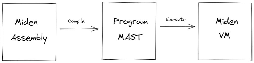
Before Miden assembly can be executed on Miden VM, it needs to be compiled into a Program MAST (Merkelized Abstract Syntax Tree) which is a binary tree of code blocks each containing raw Miden VM instructions.
As compared to raw Miden VM instructions, Miden assembly has several advantages:
- Miden assembly is intended to be a more stable external interface for the VM. That is, while we plan to make significant changes to the underlying VM to optimize it for stability, performance etc., we intend to make very few breaking changes to Miden assembly.
- Miden assembly natively supports control flow expressions which the assembler automatically transforms into a program MAST. This greatly simplifies writing programs with complex execution logic.
- Miden assembly supports macro instructions. These instructions expand into short sequences of raw Miden VM instructions making it easier to encode common operations.
- Miden assembly supports procedures. These are stand-alone blocks of code which the assembler inlines into program MAST at compile time. This improves program modularity and code organization.
The last two points also make Miden assembly much more concise as compared to the raw program MAST. This may be important in the blockchain context where pubic programs need to be stored on chain.
Terms and notations
In this document we use the following terms and notations:
- is the modulus of the VM's base field which is equal to .
- A binary value means a field element which is either or .
- Inequality comparisons are assumed to be performed on integer representations of field elements in the range .
Throughout this document, we use lower-case letters to refer to individual field elements (e.g., ). Sometimes it is convenient to describe operations over groups of elements. For these purposes we define a word to be a group of four elements. We use upper-case letters to refer to words (e.g., ). To refer to individual elements within a word, we use numerical subscripts. For example, is the first element of word , is the last element of word , etc.
Design goals
The design of Miden assembly tries to achieve the following goals:
- Miden assembly should be an easy compilation target for high-level languages.
- Programs written in Miden assembly should be readable, even if the code is generated by a compiler from a high-level language.
- Control flow should be easy to understand to help in manual inspection, formal verification, and optimization.
- Compilation of Miden assembly into Miden program MAST should be as straight-forward as possible.
- Serialization of Miden assembly into a binary representation should be as compact and as straight-forward as possible.
In order to achieve the first goal, Miden assembly exposes a set of native operations over 32-bit integers and supports linear read-write memory. Thus, from the stand-point of a higher-level language compiler, Miden VM can be viewed as a regular 32-bit stack machine with linear read-write memory.
In order to achieve the second and third goals, Miden assembly facilitates flow control via high-level constructs like while loops, if-else statements, and function calls with statically defined targets. Thus, for example, there are no explicit jump instructions.
In order to achieve the fourth goal, Miden assembly retains direct access to the VM stack rather than abstracting it away with higher-level constructs and named variables.
Lastly, in order to achieve the fifth goal, each instruction of Miden assembly can be encoded using a single byte. The resulting byte-code is simply a one-to-one mapping of instructions to their binary values.
Code organization
A Miden assembly program is just a sequence of instructions each describing a specific directive or an operation. You can use any combination of whitespace characters to separate one instruction from another.
In turn, Miden assembly instructions are just keywords which can be parameterized by zero or more parameters. The notation for specifying parameters is keyword.param1.param2 - i.e., the parameters are separated by periods. For example, push.123 instruction denotes a push operation which is parameterized by value 123.
Miden assembly programs are organized into procedures. Procedures, in turn, can be grouped into modules.
Procedures
A procedure can be used to encapsulate a frequently-used sequence of instructions which can later be invoked via a label. A procedure must start with a proc.<label>.<number of locals> instruction and terminate with an end instruction. For example:
proc.foo.2
    <instructions>
end
A procedure label must start with a letter and can contain any combination of numbers, ASCII letters, and underscores (_). Should you need to represent a label with other characters, an extended set is permitted via quoted identifiers, i.e. an identifier surrounded by "..". Quoted identifiers additionally allow any alphanumeric letter (ASCII or UTF-8), as well as various common punctuation characters: !, ?, :, ., <, >, and -. Quoted identifiers are primarily intended for representing symbols/identifiers when compiling higher-level languages to Miden Assembly, but can be used anywhere that normal identifiers are expected.
The number of locals specifies the number of memory-based local field elements a procedure can access (via loc_load, loc_store, and other instructions). If a procedure doesn't need any memory-based locals, this parameter can be omitted or set to 0. A procedure can have at most locals, and the total number of locals available to all procedures at runtime is limited to . Note that the assembler internally always rounds up the number of declared locals to the nearest multiple of 4.
To execute a procedure, the exec.<label>, call.<label>, and syscall.<label> instructions can be used. For example:
exec.foo
The difference between using each of these instructions is explained in the next section.
A procedure may execute any other procedure, however recursion is not currently permitted, due to limitations imposed by the Merkalized Abstract Syntax Tree. Recursion is caught by static analysis of the call graph during assembly, so in general you don't need to think about this, but it is a limitation to be aware of. For example, the following code block defines a program with two procedures:
proc.bar
    <instructions>
    exec.foo
    <instructions>
end

proc.foo
    <instructions>
end

begin
    <instructions>
    exec.bar
    <instructions>
    exec.foo
end
Dynamic procedure invocation
It is also possible to invoke procedures dynamically - i.e., without specifying target procedure labels at compile time. A procedure can only call itself using dynamic invocation. There are two instructions, dynexec and dyncall, which can be used to execute dynamically-specified code targets. Both instructions expect the MAST root of the target to be stored in memory, and the memory address of the MAST root to be on the top of the stack. The difference between dynexec and dyncall corresponds to the difference between exec and call, see the documentation on procedure invocation semantics for more details.
Dynamic code execution in the same context is achieved by setting the top element of the stack to the memory address where the hash of the dynamic code block is stored, and then executing the dynexec or dyncall instruction. You can obtain the hash of a procedure in the current program, by name, using the procref instruction. See the following example of pairing the two:
# Retrieve the hash of `foo`, store it at `ADDR`, and push `ADDR` on top of the stack
procref.foo mem_storew.ADDR dropw push.ADDR

# Execute `foo` dynamically
dynexec
During assembly, the procref.foo instruction is compiled to a push.HASH, where HASH is the hash of the MAST root of the foo procedure.
During execution of the dynexec instruction, the VM does the following:
- Read the top stack element , and read the memory word starting at address (the hash of the dynamic target),
- Shift the stack left by one element,
- Load the code block referenced by the hash, or trap if no such MAST root is known,
- Execute the loaded code block.
The dyncall instruction is used the same way, with the difference that it involves a context switch to a new context when executing the referenced block, and switching back to the calling context once execution of the callee completes.
Modules
A module consists of one or more procedures. There are two types of modules: library modules and executable modules (also called programs).
Library modules
Library modules contain zero or more internal procedures and one or more exported procedures. For example, the following module defines one internal procedure (defined with proc instruction) and one exported procedure (defined with export instruction):
proc.foo
    <instructions>
end

export.bar
    <instructions>
    exec.foo
    <instructions>
end
Programs
Executable modules are used to define programs. A program contains zero or more internal procedures (defined with proc instruction) and exactly one main procedure (defined with begin instruction). For example, the following module defines one internal procedure and a main procedure:
proc.foo
    <instructions>
end

begin
    <instructions>
    exec.foo
    <instructions>
end
A program cannot contain any exported procedures.
When a program is executed, the execution starts at the first instruction following the begin instruction. The main procedure is expected to be the last procedure in the program and can be followed only by comments.
Importing modules
To reference items in another module, you must either import the module you wish to use, or specify a fully-qualified path to the item you want to reference.
To import a module, you must use the use keyword in the top level scope of the current module, as shown below:
use.std::math::u64

begin
  ...
end
In this example, the std::math::u64 module is imported as u64, the default "alias" for the imported module. You can specify a different alias like so:
use.std::math::u64->bigint
This would alias the imported module as bigint rather than u64. The alias is needed to reference items from the imported module, as shown below:
use.std::math::u64

begin
    push.1.0
    push.2.0
    exec.u64::wrapping_add
end
You can also bypass imports entirely, and specify an absolute procedure path, which requires prefixing the path with ::. For example:
begin
  push.1.0
  push.2.0
  exec.::std::math::u64::wrapping_add
end
In the examples above, we have been referencing the std::math::u64 module, which is a module in the Miden Standard Library. There are a number of useful modules there, that provide a variety of helpful functionality out of the box.
If the assembler does not know about the imported modules, assembly will fail. You can register modules with the assembler when instantiating it, either in source form, or precompiled form. See the miden-assembly docs for details. The assembler will use this information to resolve references to imported procedures during assembly.
Re-exporting procedures
A procedure defined in one module can be re-exported from a different module under the same or a different name. For example:
use.std::math::u64

export.u64::add
export.u64::mul->mul64

export.foo
    <instructions>
end
In the module shown above, not only is the locally-defined procedure foo exported, but so are two procedures named add and mul64, whose implementations are defined in the std::math::u64 module.
Similar to procedure invocation, you can bypass the explicit import by specifying an absolute path, like so:
export.::std::math::u64::mul->mul64
Additionally, you may re-export a procedure using its MAST root, so long as you specify an alias:
export.0x0000..0000->mul64
In all of the forms described above, the actual implementation of the re-exported procedure is defined externally. Other modules which reference the re-exported procedure, will have those references resolved to the original procedure during assembly.
Constants
Miden assembly supports constant declarations. These constants are scoped to the module they are defined in and can be used as immediate parameters for Miden assembly instructions. Constants are supported as immediate values for many of the instructions in the Miden Assembly instruction set, see the documentation for specific instructions to determine whether or not it provides a form which accepts immediate operands.
Constants must be declared right after module imports and before any procedures or program bodies. A constant's name must start with an upper-case letter and can contain any combination of numbers, upper-case ASCII letters, and underscores (_). The number of characters in a constant name cannot exceed 100.
A constant's value must be in a decimal or hexadecimal form and be in the range between and (both inclusive). Value can be defined by an arithmetic expression using +, -, *, /, //, (, ) operators and references to the previously defined constants if it uses only decimal numbers. Here / is a field division and // is an integer division. Note that the arithmetic expression cannot contain spaces.
use.std::math::u64

const.CONSTANT_1=100
const.CONSTANT_2=200+(CONSTANT_1-50)
const.ADDR_1=3

begin
    push.CONSTANT_1.CONSTANT_2
    exec.u64::wrapping_add
    mem_store.ADDR_1
end
Comments
Miden assembly allows annotating code with simple comments. There are two types of comments: single-line comments which start with a # (pound) character, and documentation comments which start with #! characters. For example:
#! This is a documentation comment
export.foo
    # this is a comment
    push.1
end
Documentation comments must precede a procedure declaration. Using them inside a procedure body is an error.
Execution contexts
Miden assembly program execution can span multiple isolated contexts. An execution context defines its own memory space which is not accessible from other execution contexts.
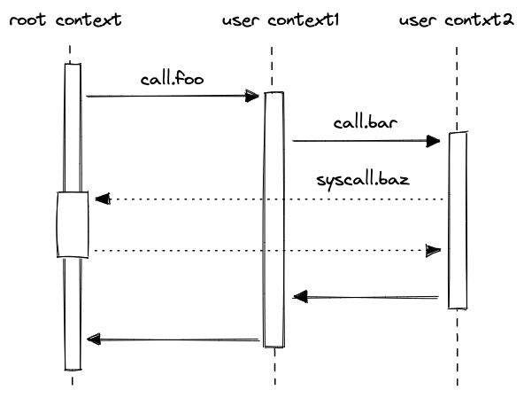
All programs start executing in a root context. Thus, the main procedure of a program is always executed in the root context. To move execution into a different context, we can invoke a procedure using the call instruction. In fact, any time we invoke a procedure using the call instruction, the procedure is executed in a new context. We refer to all non-root contexts as user contexts.
While executing in a user context, we can request to execute some procedures in the root context. This can be done via the syscall instruction. The set of procedures which can be invoked via the syscall instruction is limited by the kernel against which a program is compiled. Once the procedure called via syscall returns, the execution moves back to the user context from which it was invoked. The diagram below illustrates this graphically:
Procedure invocation semantics
As mentioned in the previous section, procedures in Miden assembly can be invoked via five different instructions: exec, call, syscall, dynexec, and dyncall. Invocation semantics of call, dyncall, and syscall instructions are basically the same, the only difference being that the syscall instruction can be used only with procedures which are defined in the program's kernel. The exec and dynexec instructions are different, and we explain these differences below.
Invoking via call, dyncall, and syscall instructions
When a procedure is invoked via a call, dyncall, or a syscall instruction, the following happens:
- Execution moves into a different context. In case of the
callanddyncallinstructions, a new user context is created. In case of asyscallinstruction, the execution moves back into the root context. - All stack items beyond the 16th item get "hidden" from the invoked procedure. That is, from the standpoint of the invoked procedure, the initial stack depth is set to 16.
- Note that for
dyncall, the stack is shifted left by one element before being set to 16.
- Note that for
When the callee returns, the following happens:
- The execution context of the caller is restored
- If the original stack depth was greater than 16, those elements that were "hidden" during the call as described above, are restored. However, the stack depth must be exactly 16 elements when the procedure returns, or this will fail and the VM will trap.
The manipulations of the stack depth described above have the following implications:
- The top 16 elements of the stack can be used to pass parameters and return values between the caller and the callee.
- Caller's stack beyond the top 16 elements is inaccessible to the callee, and thus, is guaranteed not to change as the result of the call.
- As mentioned above, in the case of
dyncall, the elements at indices 1 to 17 at the call site will be accessible to the callee (shifted to indices 0 to 16)
- As mentioned above, in the case of
- At the end of its execution, the callee must ensure that stack depth is exactly 16. If this is difficult to ensure manually, the
truncate_stackprocedure can be used to drop all elements from the stack except for the top 16.
Invoking via exec instruction
The exec instruction can be thought of as the "normal" way of invoking procedures, i.e. it has semantics that would be familiar to anyone coming from a standard programming language, or that is familiar with procedure call instructions in a typical assembly language.
In Miden Assembly, it is used to execute procedures without switching execution contexts, i.e. the callee executes in the same context as the caller. Conceptually, invoking a procedure via exec behaves as if the body of that procedure was inlined at the call site. In practice, the procedure may or may not be actually inlined, based on compiler optimizations around code size, but there is no actual performance tradeoff in the usual sense. Thus, when executing a program, there is no meaningful difference between executing a procedure via exec, or replacing the exec with the body of the procedure.
Kernels
A kernel defines a set of procedures which can be invoked from user contexts to be executed in the root context. Miden assembly programs are always compiled against some kernel. The default kernel is empty - i.e., it does not contain any procedures. To compile a program against a non-empty kernel, the kernel needs to be specified when instantiating the Miden Assembler.
A kernel can be defined similarly to a regular library module - i.e., it can have internal and exported procedures. However, there are some small differences between what procedures can do in a kernel module vs. what they can do in a regular library module. Specifically:
- Procedures in a kernel module cannot use
call,dyncallorsyscallinstructions. This means that creating a new context from within asyscallis not possible. - Unlike procedures in regular library modules, procedures in a kernel module can use the
callerinstruction. This instruction puts the hash of the procedure which initiated the parent context onto the stack.
Memory layout
As mentioned earlier, procedures executed within a given context can access memory only of that context. This is true for both memory reads and memory writes.
Address space of every context is the same: the smallest accessible address is and the largest accessible address is . Any code executed in a given context has access to its entire address space. However, by convention, we assign different meanings to different regions of the address space.
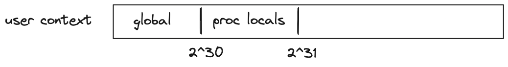
For user contexts we have the following:
- The first addresses are assumed to be global memory.
- The next addresses are reserved for memory locals of procedures executed in the same context (i.e., via the
execinstruction). - The remaining address space has no special meaning.
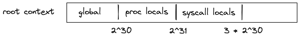
For the root context we have the following:
- The first addresses are assumed to be global memory.
- The next addresses are reserved for memory locals of procedures executed in the root context.
- The next addresses are reserved for memory locals of procedures executed from within a
syscall. - The remaining address space has no special meaning.
For both types of contexts, writing directly into regions of memory reserved for procedure locals is not advisable. Instead, loc_load, loc_store and other similar dedicated instructions should be used to access procedure locals.
Example
To better illustrate what happens as we execute procedures in different contexts, let's go over the following example.
kernel
--------------------
export.baz.2
    <instructions>
    caller
    <instructions>
end

program
--------------------
proc.bar.1
    <instructions>
    syscall.baz
    <instructions>
end

proc.foo.3
    <instructions>
    call.bar
    <instructions>
    exec.bar
    <instructions>
end

begin
    <instructions>
    call.foo
    <instructions>
end
Execution of the above program proceeds as follows:
- The VM starts executing instructions immediately following the
beginstatement. These instructions are executed in the root context (let's call this contextctx0). - When
call.foois executed, a new context is created (ctx1). Memory in this context is isolated fromctx0. Additionally, any elements on the stack beyond the top 16 are hidden fromfoo. - Instructions executed inside
foocan access memory ofctx1only. The address of the first procedure local infoo(e.g., accessed vialoc_load.0) is . - When
call.baris executed, a new context is created (ctx2). The stack depth is set to 16 again, and any instruction executed in this context can access memory ofctx2only. The first procedure local ofbaris also located at address . - When
syscall.bazis executed, the execution moves back into the root context. That is, instructions executed insidebazhave access to the memory ofctx0. The first procedure local ofbazis located at address . Whenbazstarts executing, the stack depth is again set to 16. - When
calleris executed insidebaz, the first 4 elements of the stack are populated with the hash ofbarsincebazwas invoked frombar's context. - Once
bazreturns, execution moves back toctx2, and then, whenbarreturns, execution moves back toctx1. We assume that instructions executed right before each procedure returns ensure that the stack depth is exactly 16 right before procedure's end. - Next, when
exec.baris executed,baris executed again, but this time it is executed in the same context asfoo. Thus, it can access memory ofctx1. Moreover, the stack depth is not changed, and thus,barcan access the entire stack offoo. Lastly, this first procedure local ofbarnow will be at address (since the first 3 locals in this context are reserved forfoo). - When
syscall.bazis executed the second time, execution moves into the root context again. However, now, whencalleris executed insidebaz, the first 4 elements of the stack are populated with the hash offoo(notbar). This happens because this time aroundbardoes not have its own context andbazis invoked fromfoo's context. - Finally, when
bazreturns, execution moves back toctx1, and then asbarandfooreturn, back toctx0, and the program terminates.
Flow control
As mentioned above, Miden assembly provides high-level constructs to facilitate flow control. These constructs are:
- if-else expressions for conditional execution.
- repeat expressions for bounded counter-controlled loops.
- while expressions for unbounded condition-controlled loops.
Conditional execution
Conditional execution in Miden VM can be accomplished with if-else statements. These statements can take one of the following forms:
if.true .. else .. end
This is the full form, when there is work to be done on both branches:
if.true
  ..instructions..
else
  ..instructions..
end
if.true .. end
This is the abbreviated form, for when there is only work to be done on one branch. In these cases the "unused" branch can be elided:
if.true
  ..instructions..
end
In addition to if.true, there is also if.false, which is identical in syntax, but for false-conditioned branches. It is equivalent in semantics to using if.true and swapping the branches.
The body of each branch, i.e. ..instructions.. in the examples above, can be a sequence of zero or more instructions (an empty body is only valid so long as at least one branch is non-empty). These can consist of any instruction, including nested control flow.
tip
As with other control structures described below that have nested blocks,
it is essential that you ensure that the state of the operand stack is
consistent at join points in control flow. For example, with if.true
control flow implicitly joins at the end of each branch. If you have moved
items around on the operand stack, or added/removed items, and those
modifications would persist past the end of that branch, it is highly
recommended that you make equivalent modifications in the opposite branch.
This is not required if modifications are local to a block.
The semantics of the if.true and if.false control operator are as follows:
- The condition is popped from the top of the stack. It must be a boolean value, i.e. for false, for true. If the condition is not a boolean value, then execution traps.
- The conditional branch is chosen:
a. If the operator is
if.true, and the condition is true, instructions in the first branch are executed; otherwise, if the condition is false, then the second branch is executed. If a branch was elided or empty, the assembler provides a default body consisting of a singlenopinstruction. b. If the operator isif.false, the behavior is identical to that ofif.true, except the condition must be false for the first branch to be taken, and true for the second branch. - Control joins at the next instruction immediately following the
if.true/if.falseinstruction.
tip
A note on performance: using if-else statements incurs a small, but non-negligible overhead. Thus, for simple conditional statements, it may be more efficient to compute the result of both branches, and then select the result using conditional drop instructions.
This does not apply to if-else statements whose bodies contain side-effects that cannot be easily adapted to this type of rewrite. For example, writing a value to global memory is a side effect, but if both branches would write to the same address, and only the value being written differs, then this can likely be rewritten to use cdrop.
Counter-controlled loops
Executing a sequence of instructions a predefined number of times can be accomplished with repeat statements. These statements look like so:
repeat.<count>
    <instructions>
end
where:
instructionscan be a sequence of any instructions, including nested control structures.countis the number of times theinstructionssequence should be repeated (e.g.repeat.10).countmust be an integer or a constant greater than .
Note: During compilation the
repeat.<count>blocks are unrolled and expanded into<count>copies of its inner block, there is no additional cost for counting variables in this case.
Condition-controlled loops
Executing a sequence of instructions zero or more times based on some condition can be accomplished with while loop expressions. These expressions look like so:
while.true
    <instructions>
end
where instructions can be a sequence of any instructions, including nested control structures. The above does the following:
- Pops the top item from the stack.
- If the value of the item is ,
instructionsin the loop body are executed.- After the body is executed, the stack is popped again, and if the popped value is , the body is executed again.
- If the popped value is , the loop is exited.
- If the popped value is not binary, the execution fails.
- If the value of the item is , execution of loop body is skipped.
- If the value is not binary, the execution fails.
Example:
# push the boolean true to the stack
push.1

# pop the top element of the stack and loop while it is true
while.true
    # push the boolean false to the stack, finishing the loop for the next iteration
    push.0
end
No-op
While rare, there may be situations where you have an empty block and require a do-nothing placeholder instruction, or where you specifically want to advance the cycle counter without any side-effects. The nop instruction can be used in these instances.
if.true
  nop
else
  ..instructions..
end
In the example above, we do not want to perform any work if the condition is true, so we place a nop in that branch. This explicit representation of "empty" blocks is automatically done by the assembler when parsing if.true or if.false in abbreviated form, or when one of the branches is empty.
The semantics of this instruction are to increment the cycle count, and that is it - no other effects.
Field operations
Miden assembly provides a set of instructions which can perform operations with raw field elements. These instructions are described in the tables below.
While most operations place no restrictions on inputs, some operations expect inputs to be binary values, and fail if executed with non-binary inputs.
For instructions where one or more operands can be provided as immediate parameters (e.g., add and add.b), we provide stack transition diagrams only for the non-immediate version. For the immediate version, it can be assumed that the operand with the specified name is not present on the stack.
Assertions and tests
| Instruction | Stack_input | Stack_output | Notes |
|---|---|---|---|
| assert - (1 cycle) | [a, ...] | [...] | If , removes it from the stack. Fails if |
| assertz - (2 cycles) | [a, ...] | [...] | If , removes it from the stack, Fails if |
| assert_eq - (2 cycles) | [b, a, ...] | [...] | If , removes them from the stack. Fails if |
| assert_eqw - (11 cycles) | [B, A, ...] | [...] | If , removes them from the stack. Fails if |
The above instructions can also be parametrized with an error code which can be any 32-bit value specified either directly or via a named constant. For example:
assert.err=123
assert.err=MY_CONSTANT
If the error code is omitted, the default value of is assumed.
Arithmetic and Boolean operations
The arithmetic operations below are performed in a 64-bit prime field defined by modulus . This means that overflow happens after a value exceeds . Also, the result of divisions may appear counter-intuitive because divisions are defined via inversions.
| Instruction | Stack_input | Stack_output | Notes |
|---|---|---|---|
| add - (1 cycle) add.b - (1-2 cycle) | [b, a, ...] | [c, ...] | |
| sub - (2 cycles) sub.b - (2 cycles) | [b, a, ...] | [c, ...] | |
| mul - (1 cycle) mul.b - (2 cycles) | [b, a, ...] | [c, ...] | |
| div - (2 cycles) div.b - (2 cycles) | [b, a, ...] | [c, ...] | Fails if |
| neg - (1 cycle) | [a, ...] | [b, ...] | |
| inv - (1 cycle) | [a, ...] | [b, ...] | Fails if |
| pow2 - (16 cycles) | [a, ...] | [b, ...] | Fails if |
| exp.uxx - (9 + xx cycles) exp.b - (9 + log2(b) cycles) | [b, a, ...] | [c, ...] | Fails if xx is outside [0, 63) exp is equivalent to exp.u64 and needs 73 cycles |
| ilog2 - (44 cycles) | [a, ...] | [b, ...] | Fails if |
| not - (1 cycle) | [a, ...] | [b, ...] | Fails if |
| and - (1 cycle) | [b, a, ...] | [c, ...] | Fails if |
| or - (1 cycle) | [b, a, ...] | [c, ...] | Fails if |
| xor - (7 cycles) | [b, a, ...] | [c, ...] | Fails if |
Comparison operations
| Instruction | Stack_input | Stack_output | Notes |
|---|---|---|---|
| eq - (1 cycle) eq.b - (1-2 cycles) | [b, a, ...] | [c, ...] | |
| neq - (2 cycle) neq.b - (2-3 cycles) | [b, a, ...] | [c, ...] | |
| lt - (14 cycles) lt.b - (15 cycles) | [b, a, ...] | [c, ...] | |
| lte - (15 cycles) lte.b - (16 cycles) | [b, a, ...] | [c, ...] | |
| gt - (15 cycles) gt.b - (16 cycles) | [b, a, ...] | [c, ...] | |
| gte - (16 cycles) gte.b - (17 cycles) | [b, a, ...] | [c, ...] | |
| is_odd - (5 cycles) | [a, ...] | [b, ...] | |
| eqw - (15 cycles) | [A, B, ...] | [c, A, B, ...] |
Extension Field Operations
| Instruction | Stack_input | Stack_output | Notes |
|---|---|---|---|
| ext2add - (5 cycles) | [b1, b0, a1, a0, ...] | [c1, c0, ...] | and |
| ext2sub - (7 cycles) | [b1, b0, a1, a0, ...] | [c1, c0, ...] | and |
| ext2mul - (3 cycles) | [b1, b0, a1, a0, ...] | [c1, c0, ...] | and |
| ext2neg - (4 cycles) | [a1, a0, ...] | [a1', a0', ...] | and |
| ext2inv - (8 cycles) | [a1, a0, ...] | [a1', a0', ...] | Fails if |
| ext2div - (11 cycles) | [b1, b0, a1, a0, ...] | [c1, c0,] | fails if , where multiplication and inversion are as defined by the operations above |
u32 operations
Miden assembly provides a set of instructions which can perform operations on regular two-complement 32-bit integers. These instructions are described in the tables below.
For instructions where one or more operands can be provided as immediate parameters (e.g., u32wrapping_add and u32wrapping_add.b), we provide stack transition diagrams only for the non-immediate version. For the immediate version, it can be assumed that the operand with the specified name is not present on the stack.
In all the table below, the number of cycles it takes for the VM to execute each instruction is listed beneath the instruction.
Notes on Undefined Behavior
Most of the instructions documented below expect to receive operands whose values are valid u32
values, i.e. values in the range . Currently, the semantics of the instructions
when given values outside of that range are undefined (as noted in the documented semantics for
each instruction). The rule with undefined behavior generally speaking is that you can make no
assumptions about what will happen if your program exhibits it.
For purposes of describing the effects of undefined behavior below, we will refer to values which
are not valid for the input type of the affected operation, e.g. u32, as poison. Any use of a
poison value propagates the poison state. For example, performing u32div with a poison operand,
can be considered as producing a poison value as its result, for the purposes of discussing
undefined behavior semantics.
With that in mind, there are two ways in which the effects of undefined behavior manifest:
Executor Semantics
From an executor perspective, currently, the semantics are completely undefined. An executor can do everything from terminate the program, panic, always produce 42 as a result, produce a random result, or something more principled.
In practice, the Miden VM, when executing an operation, will almost always trap on poison values. This is not guaranteed, but is currently the case for most operations which have niches of undefined behavior. To the extent that some other behavior may occur, it will generally be to truncate/wrap the poison value, but this is subject to change at any time, and is undocumented. You should assume that all operations will trap on poison.
The reason the Miden VM makes the choice to trap on poison, is to ensure that undefined behavior is caught close to the source, rather than propagated silently throughout the program. It also has the effect of ensuring you do not execute a program with undefined behavior, and produce a proof that is not actually valid, as we will describe in a moment.
Verifier Semantics
From the perspective of the verifier, the implementation details of the executor are completely unknown. For example, the fact that the Miden VM traps on poison values is not actually verified by constraints. An alternative executor implementation could choose not to trap, and thus appear to execute successfully. The resulting proof, however, as a result of the program exhibiting undefined behavior, is not a valid proof. In effect the use of poison values "poisons" the proof as well.
As a result, a program that exhibits undefined behavior, and executes successfully, will produce a proof that could pass verification, even though it should not. In other words, the proof does not prove what it says it does.
In the future, we may attempt to remove niches of undefined behavior in such a way that producing such invalid proofs is not possible, but for the time being, you must ensure that your program does not exhibit (or rely on) undefined behavior.
Conversions and tests
| Instruction | Stack_input | Stack_output | Notes |
|---|---|---|---|
| u32test - (5 cycles) | [a, ...] | [b, a, ...] | |
| u32testw - (23 cycles) | [A, ...] | [b, A, ...] | |
| u32assert - (3 cycles) | [a, ...] | [a, ...] | Fails if |
| u32assert2 - (1 cycle) | [b, a,...] | [b, a,...] | Fails if or |
| u32assertw - (6 cycles) | [A, ...] | [A, ...] | Fails if |
| u32cast - (2 cycles) | [a, ...] | [b, ...] | |
| u32split - (1 cycle) | [a, ...] | [c, b, ...] | , |
The instructions u32assert, u32assert2 and u32assertw can also be parametrized with an error code which can be any 32-bit value specified either directly or via a named constant. For example:
u32assert.err=123
u32assert.err=MY_CONSTANT
If the error code is omitted, the default value of is assumed.
Arithmetic operations
| Instruction | Stack_input | Stack_output | Notes |
|---|---|---|---|
| u32overflowing_add - (1 cycle) u32overflowing_add.b - (2-3 cycles) | [b, a, ...] | [d, c, ...] | Undefined if |
| u32wrapping_add - (2 cycles) u32wrapping_add.b - (3-4 cycles) | [b, a, ...] | [c, ...] | Undefined if |
| u32overflowing_add3 - (1 cycle) | [c, b, a, ...] | [e, d, ...] | , Undefined if |
| u32wrapping_add3 - (2 cycles) | [c, b, a, ...] | [d, ...] | , Undefined if |
| u32overflowing_sub - (1 cycle) u32overflowing_sub.b - (2-3 cycles) | [b, a, ...] | [d, c, ...] | Undefined if |
| u32wrapping_sub - (2 cycles) u32wrapping_sub.b - (3-4 cycles) | [b, a, ...] | [c, ...] | Undefined if |
| u32overflowing_mul - (1 cycle) u32overflowing_mul.b - (2-3 cycles) | [b, a, ...] | [d, c, ...] | Undefined if |
| u32wrapping_mul - (2 cycles) u32wrapping_mul.b - (3-4 cycles) | [b, a, ...] | [c, ...] | Undefined if |
| u32overflowing_madd - (1 cycle) | [b, a, c, ...] | [e, d, ...] | Undefined if |
| u32wrapping_madd - (2 cycles) | [b, a, c, ...] | [d, ...] | Undefined if |
| u32div - (2 cycles) u32div.b - (3-4 cycles) | [b, a, ...] | [c, ...] | Fails if Undefined if |
| u32mod - (3 cycles) u32mod.b - (4-5 cycles) | [b, a, ...] | [c, ...] | Fails if Undefined if |
| u32divmod - (1 cycle) u32divmod.b - (2-3 cycles) | [b, a, ...] | [d, c, ...] | Fails if Undefined if |
Bitwise operations
| Instruction | Stack_input | Stack_output | Notes |
|---|---|---|---|
| u32and - (1 cycle) u32and.b - (2 cycles) | [b, a, ...] | [c, ...] | Computes as a bitwise AND of binary representations of and . Fails if |
| u32or - (6 cycle)s u32or.b - (7 cycles) | [b, a, ...] | [c, ...] | Computes as a bitwise OR of binary representations of and . Fails if |
| u32xor - (1 cycle) u32xor.b - (2 cycles) | [b, a, ...] | [c, ...] | Computes as a bitwise XOR of binary representations of and . Fails if |
| u32not - (5 cycles) u32not.a - (6 cycles) | [a, ...] | [b, ...] | Computes as a bitwise NOT of binary representation of . Fails if |
| u32shl - (18 cycles) u32shl.b - (3 cycles) | [b, a, ...] | [c, ...] | Undefined if or |
| u32shr - (18 cycles) u32shr.b - (3 cycles) | [b, a, ...] | [c, ...] | Undefined if or |
| u32rotl - (18 cycles) u32rotl.b - (3 cycles) | [b, a, ...] | [c, ...] | Computes by rotating a 32-bit representation of to the left by bits. Undefined if or |
| u32rotr - (23 cycles) u32rotr.b - (3 cycles) | [b, a, ...] | [c, ...] | Computes by rotating a 32-bit representation of to the right by bits. Undefined if or |
| u32popcnt - (33 cycles) | [a, ...] | [b, ...] | Computes by counting the number of set bits in (hamming weight of ). Undefined if |
| u32clz - (42 cycles) | [a, ...] | [b, ...] | Computes as a number of leading zeros of . Undefined if |
| u32ctz - (34 cycles) | [a, ...] | [b, ...] | Computes as a number of trailing zeros of . Undefined if |
| u32clo - (41 cycles) | [a, ...] | [b, ...] | Computes as a number of leading ones of . Undefined if |
| u32cto - (33 cycles) | [a, ...] | [b, ...] | Computes as a number of trailing ones of . Undefined if |
Comparison operations
| Instruction | Stack_input | Stack_output | Notes |
|---|---|---|---|
| u32lt - (3 cycles) u32lt.b - (4 cycles) | [b, a, ...] | [c, ...] | Undefined if |
| u32lte - (5 cycles) u32lte.b - (6 cycles) | [b, a, ...] | [c, ...] | Undefined if |
| u32gt - (4 cycles) u32gt.b - (5 cycles) | [b, a, ...] | [c, ...] | Undefined if |
| u32gte - (4 cycles) u32gte.b - (5 cycles) | [b, a, ...] | [c, ...] | Undefined if |
| u32min - (8 cycles) u32min.b - (9 cycles) | [b, a, ...] | [c, ...] | Undefined if |
| u32max - (9 cycles) u32max.b - (10 cycles) | [b, a, ...] | [c, ...] | Undefined if |
Stack manipulation
Miden VM stack is a push-down stack of field elements. The stack has a maximum depth of , but only the top elements are directly accessible via the instructions listed below.
In addition to the typical stack manipulation instructions such as drop, dup, swap etc., Miden assembly provides several conditional instructions which can be used to manipulate the stack based on some condition - e.g., conditional swap cswap or conditional drop cdrop.
| Instruction | Stack_input | Stack_output | Notes |
|---|---|---|---|
| drop - (1 cycle) | [a, ... ] | [ ... ] | Deletes the top stack item. |
| dropw - (4 cycles) | [A, ... ] | [ ... ] | Deletes a word (4 elements) from the top of the stack. |
| padw - (4 cycles) | [ ... ] | [0, 0, 0, 0, ... ] | Pushes four values onto the stack. Note: simple pad is not provided because push.0 does the same thing. |
| dup.n - (1-3 cycles) | [ ..., a, ... ] | [a, ..., a, ... ] | Pushes a copy of the th stack item onto the stack. dup and dup.0 are the same instruction. Valid for |
| dupw.n - (4 cycles) | [ ..., A, ... ] | [A, ..., A, ... ] | Pushes a copy of the th stack word onto the stack. dupw and dupw.0 are the same instruction. Valid for |
| swap.n - (1-6 cycles) | [a, ..., b, ... ] | [b, ..., a, ... ] | Swaps the top stack item with the th stack item. swap and swap.1 are the same instruction. Valid for |
| swapw.n - (1 cycle) | [A, ..., B, ... ] | [B, ..., A, ... ] | Swaps the top stack word with the th stack word. swapw and swapw.1 are the same instruction. Valid for |
| swapdw - (1 cycle) | [D, C, B, A, ... ] | [B, A, D, C ... ] | Swaps words on the top of the stack. The 1st with the 3rd, and the 2nd with the 4th. |
| movup.n - (1-4 cycles) | [ ..., a, ... ] | [a, ... ] | Moves the th stack item to the top of the stack. Valid for |
| movupw.n - (2-3 cycles) | [ ..., A, ... ] | [A, ... ] | Moves the th stack word to the top of the stack. Valid for |
| movdn.n - (1-4 cycles) | [a, ... ] | [ ..., a, ... ] | Moves the top stack item to the th position of the stack. Valid for |
| movdnw.n - (2-3 cycles) | [A, ... ] | [ ..., A, ... ] | Moves the top stack word to the th word position of the stack. Valid for |
Conditional manipulation
| Instruction | Stack_input | Stack_output | Notes |
|---|---|---|---|
| cswap - (1 cycle) | [c, b, a, ... ] | [e, d, ... ] | Fails if |
| cswapw - (1 cycle) | [c, B, A, ... ] | [E, D, ... ] | Fails if |
| cdrop - (2 cycles) | [c, b, a, ... ] | [d, ... ] | Fails if |
| cdropw - (5 cycles) | [c, B, A, ... ] | [D, ... ] | Fails if |
Input / output operations
Miden assembly provides a set of instructions for moving data between the operand stack and several other sources. These sources include:
- Program code: values to be moved onto the operand stack can be hard-coded in a program's source code.
- Environment: values can be moved onto the operand stack from environment variables. These include current clock cycle, current stack depth, and a few others.
- Advice provider: values can be moved onto the operand stack from the advice provider by popping them from the advice stack (see more about the advice provider here). The VM can also inject new data into the advice provider via system event instructions.
- Memory: values can be moved between the stack and random-access memory. The memory is element-addressable, meaning that a single element is located at each address. However, reading and writing elements to/from memory in batches of four is supported via the appropriate instructions (e.g.
mem_loadwormem_storew). Memory can be accessed via absolute memory references (i.e., via memory addresses) as well as via local procedure references (i.e., local index). The latter approach ensures that a procedure does not access locals of another procedure.
Constant inputs
| Instruction | Stack_input | Stack_output | Notes |
|---|---|---|---|
| push.a - (1-2 cycles) push.a.b push.a.b.c... | [ ... ] | [a, ... ] [b, a, ... ] [c, b, a, ... ] | Pushes values , , etc. onto the stack. Up to values can be specified. All values must be valid field elements in decimal (e.g., ) or hexadecimal (e.g., ) representation. |
The value can be specified in hexadecimal form without periods between individual values as long as it describes a full word ( field elements or bytes). Note that hexadecimal values separated by periods (short hexadecimal strings) are assumed to be in big-endian order, while the strings specifying whole words (long hexadecimal strings) are assumed to be in little-endian order. That is, the following are semantically equivalent:
push.0x00001234.0x00005678.0x00009012.0x0000abcd
push.0x341200000000000078560000000000001290000000000000cdab000000000000
push.4660.22136.36882.43981
In both case the values must still encode valid field elements.
Environment inputs
| Instruction | Stack_input | Stack_output | Notes |
|---|---|---|---|
| clk - (1 cycle) | [ ... ] | [t, ... ] | Pushes the current value of the clock cycle counter onto the stack. |
| sdepth - (1 cycle) | [ ... ] | [d, ... ] | Pushes the current depth of the stack onto the stack. |
| caller - (1 cycle) | [A, b, ... ] | [H, b, ... ] | Overwrites the top four stack items with the hash of a function which initiated the current SYSCALL. Executing this instruction outside of SYSCALL context will fail. |
| locaddr.i - (2 cycles) | [ ... ] | [a, ... ] | Pushes the absolute memory address of local memory at index onto the stack. |
| procref.name - (4 cycles) | [ ... ] | [A, ... ] | Pushes MAST root of the procedure with name onto the stack. |
Nondeterministic inputs
As mentioned above, nondeterministic inputs are provided to the VM via the advice provider. Instructs which access the advice provider fall into two categories. The first category consists of instructions which move data from the advice stack onto the operand stack and/or memory.
| Instruction | Stack_input | Stack_output | Notes |
|---|---|---|---|
| adv_push.n - (n cycles) | [ ... ] | [a, ... ] | Pops values from the advice stack and pushes them onto the operand stack. Valid for . Fails if the advice stack has fewer than values. |
| adv_loadw - (1 cycle) | [0, 0, 0, 0, ... ] | [A, ... ] | Pop the next word (4 elements) from the advice stack and overwrites the first word of the operand stack (4 elements) with them. Fails if the advice stack has fewer than values. |
| adv_pipe - (1 cycle) | [C, B, A, a, ... ] | [E, D, A, a', ... ] | Pops the next two words from the advice stack, overwrites the top of the operand stack with them and also writes these words into memory at address and . Fails if the advice stack has fewer than values. |
Note: The opcodes above always push data onto the operand stack so that the first element is placed deepest in the stack. For example, if the data on the stack is
a,b,c,dand you use the opcodeadv_push.4, the data will bed,c,b,aon your stack. This is also the behavior of the other opcodes.
The second category injects new data into the advice provider. These operations are called system events and they affect only the advice provider state. That is, the state of all other VM components (e.g., stack, memory) are unaffected. Handling system events does not consume any VM cycles (i.e., these instructions are executed in cycles).
System events fall into two categories: (1) events which push new data onto the advice stack, and (2) events which insert new data into the advice map.
| Instruction | Stack_input | Stack_output | Notes |
|---|---|---|---|
| adv.push_mapval | [K, ... ] | [K, ... ] | Pushes a list of field elements onto the advice stack. The list is looked up in the advice map using word as the key. |
| adv.push_mapvaln | [K, ... ] | [K, ... ] | Pushes a list of field elements together with the number of elements onto the advice stack ([n, ele1, ele2, ...], where n is the number of elements pushed). The list is looked up in the advice map using word as the key. |
| adv.push_mtnode | [d, i, R, ... ] | [d, i, R, ... ] | Pushes a node of a Merkle tree with root at depth and index from Merkle store onto the advice stack. |
| adv.push_u64div | [b1, b0, a1, a0, ...] | [b1, b0, a1, a0, ...] | Pushes the result of u64 division onto the advice stack. Both and are represented using 32-bit limbs. The result consists of both the quotient and the remainder. |
| adv.push_ext2intt | [osize, isize, iptr, ... ] | [osize, isize, iptr, ... ] | Given evaluations of a polynomial over some specified domain, interpolates the evaluations into a polynomial in coefficient form and pushes the result into the advice stack. |
| adv.push_smtpeek | [K, R, ... ] | [K, R, ... ] | Pushes value onto the advice stack which is associated with key in a Sparse Merkle Tree with root . |
| adv.insert_mem | [K, a, b, ... ] | [K, a, b, ... ] | Reads words from memory, and save the data into . |
| adv.insert_hdword | [B, A, ... ] | [B, A, ... ] | Reads top two words from the stack, computes a key as , and saves the data into . |
| adv.insert_hdword_d | [B, A, d, ... ] | [B, A, d, ... ] | Reads top two words from the stack, computes a key as , and saves the data into . is the domain value, where changing the domain changes the resulting hash given the same A and B. |
| adv.insert_hperm | [B, A, C, ...] | [B, A, C, ...] | Reads top three words from the stack, computes a key as , and saves data into . |
Random access memory
As mentioned above, there are two ways to access memory in Miden VM. The first way is via memory addresses using the instructions listed below. The addresses are absolute - i.e., they don't depend on the procedure context. Memory addresses can be in the range .
Memory is guaranteed to be initialized to zeros. Thus, when reading from memory address which hasn't been written to previously, zero elements will be returned.
| Instruction | Stack_input | Stack_output | Notes |
|---|---|---|---|
| mem_load - (1 cycle) mem_load.a - (2 cycles) | [a, ... ] | [v, ... ] | Reads the field element from memory at address a, and pushes it onto the stack. If is provided via the stack, it is removed from the stack first. Fails if |
| mem_loadw - (1 cycle) mem_loadw.a - (2 cycles) | [a, 0, 0, 0, 0, ... ] | [A, ... ] | Reads a word from memory starting at address and overwrites top four stack elements with it, in reverse order, such that mem[a+3] is on top of the stack. If is provided via the stack, it is removed from the stack first. Fails if , or if is not a multiple of 4 |
| mem_store - (2 cycles) mem_store.a - (3-4 cycles) | [a, v, ... ] | [ ... ] | Pops the top element off the stack and stores it in memory at address . If is provided via the stack, it is removed from the stack first. Fails if |
| mem_storew - (1 cycle) mem_storew.a - (2-3 cycles) | [a, A, ... ] | [A, ... ] | Stores the top four elements of the stack in reverse order in memory starting at address , such that the first element of A is placed at mem[a+3]. If is provided via the stack, it is removed from the stack first. Fails if , or if is not a multiple of 4 |
| mem_stream - (1 cycle) | [C, B, A, a, ... ] | [E, D, A, a', ... ] | Read two sequential words from memory starting at address and overwrites the first two words in the operand stack. |
The second way to access memory is via procedure locals using the instructions listed below. These instructions are available only in procedure context. The number of locals available to a given procedure must be specified at procedure declaration time, and trying to access more locals than was declared will result in a compile-time error. A procedure can have at most locals, and the total number of locals available to all procedures at runtime is limited to . The assembler internally always rounds up the number of declared locals to the nearest multiple of 4.
| Instruction | Stack_input | Stack_output | Notes |
|---|---|---|---|
| loc_load.i - (3-4 cycles) | [ ... ] | [v, ... ] | Reads a field element from local memory at index i, and pushes it onto the stack. |
| loc_loadw.i - (3-4 cycles) | [0, 0, 0, 0, ... ] | [A, ... ] | Reads a word from local memory starting at index and overwrites top four stack elements with it in reverse order, such that local[i+3] is placed at the top of the stack. Fails if is not a multiple 4. |
| loc_store.i - (4-5 cycles) | [v, ... ] | [ ... ] | Pops the top element off the stack and stores it in local memory at index . |
| loc_storew.i - (3-4 cycles) | [A, ... ] | [A, ... ] | Stores the top four elements of the stack in local memory in reverse order starting at index , such that the top of stack is placed at local[i+3]. |
Unlike regular memory, procedure locals are not guaranteed to be initialized to zeros. Thus, when working with locals, one must assume that before a local memory address has been written to, it contains "garbage".
Internally in the VM, procedure locals are stored at memory offset starting at . Thus, every procedure local has an absolute address in regular memory. The locaddr.i instruction is provided specifically to map an index of a procedure's local to an absolute address so that it can be passed to downstream procedures, when needed.
Cryptographic operations
Miden assembly provides a set of instructions for performing common cryptographic operations. These instructions are listed in the table below.
Hashing and Merkle trees
Rescue Prime Optimized is the native hash function of Miden VM. The parameters of the hash function were chosen to provide 128-bit security level against preimage and collision attacks. The function operates over a state of 12 field elements, and requires 7 rounds for a single permutation. However, due to its special status within the VM, computing Rescue Prime Optimized hashes can be done very efficiently. For example, applying a permutation of the hash function can be done in a single VM cycle.
| Instruction | Stack_input | Stack_output | Notes |
|---|---|---|---|
| hash - (20 cycles) | [A, ...] | [B, ...] | where, computes a 1-to-1 Rescue Prime Optimized hash. |
| hperm - (1 cycle) | [C, B, A, ...] | [F, E, D, ...] | Performs a Rescue Prime Optimized permutation on the top 3 words of the operand stack, where the top 2 words elements are the rate (words C and B), the deepest word is the capacity (word A), the digest output is the word E. |
| hmerge - (16 cycles) | [B, A, ...] | [C, ...] | where, computes a 2-to-1 Rescue Prime Optimized hash. |
| mtree_get - (9 cycles) | [d, i, R, ...] | [V, R, ...] | Fetches the node value from the advice provider and runs a verification equivalent to mtree_verify, returning the value if succeeded. |
| mtree_set - (29 cycles) | [d, i, R, V', ...] | [V, R', ...] | Updates a node in the Merkle tree with root at depth and index to value . is the Merkle root of the resulting tree and is old value of the node. Merkle tree with root must be present in the advice provider, otherwise execution fails. At the end of the operation the advice provider will contain both Merkle trees. |
| mtree_merge - (16 cycles) | [R, L, ...] | [M, ...] | Merges two Merkle trees with the provided roots R (right), L (left) into a new Merkle tree with root M (merged). The input trees are retained in the advice provider. |
| mtree_verify - (1 cycle) | [V, d, i, R, ...] | [V, d, i, R, ...] | Verifies that a Merkle tree with root opens to node at depth and index . Merkle tree with root must be present in the advice provider, otherwise execution fails. |
The mtree_verify instruction can also be parametrized with an error code which can be any 32-bit value specified either directly or via a named constant. For example:
mtree_verify.err=123
mtree_verify.err=MY_CONSTANT
If the error code is omitted, the default value of is assumed.
Events
Miden assembly supports the concept of events. Events are a simple data structure with a single event_id field. When an event is emitted by a program, it is communicated to the host. Events can be emitted at specific points of program execution with the intent of triggering some action on the host. This is useful as the program has contextual information that would be challenging for the host to infer. The emission of events allows the program to communicate this contextual information to the host. The host contains an event handler that is responsible for handling events and taking appropriate actions. The emission of events does not change the state of the VM but it can change the state of the host.
An event can be emitted via the emit.<event_id> assembly instruction where <event_id> can be any 32-bit value specified either directly or via a named constant. For example:
emit.EVENT_ID_1
emit.2
Tracing
Miden assembly also supports code tracing, which works similar to the event emitting.
A trace can be emitted via the trace.<trace_id> assembly instruction where <trace_id> can be any 32-bit value specified either directly or via a named constant. For example:
trace.EVENT_ID_1
trace.2
To make use of the trace instruction, programs should be ran with tracing flag (-t or --trace), otherwise these instructions will be ignored.
Debugging
To support basic debugging capabilities, Miden assembly provides a debug instruction. This instruction prints out the state of the VM at the time when the debug instruction is executed. The instruction can be parameterized as follows:
debug.stackprints out the entire contents of the stack.debug.stack.<n>prints out the top items of the stack. must be an integer greater than and smaller than .debug.memprints out the entire contents of RAM.debug.mem.<n>prints out contents of memory at address .debug.mem.<n>.<m>prints out the contents of memory starting at address and ending at address (both inclusive). must be greater or equal to .debug.localprints out the whole local memory of the currently executing procedure.debug.local.<n>prints out contents of the local memory at index for the currently executing procedure. must be greater or equal to and smaller than .debug.local.<n>.<m>prints out contents of the local memory starting at index and ending at index (both inclusive). must be greater or equal to . and must be greater or equal to and smaller than .
Debug instructions do not affect the VM state and do not change the program hash.
To make use of the debug instruction, programs must be compiled with an assembler instantiated in the debug mode. Otherwise, the assembler will simply ignore the debug instructions.
Miden Standard Library
Miden standard library provides a set of procedures which can be used by any Miden program. These procedures build on the core instruction set of Miden assembly expanding the functionality immediately available to the user.
The goals of Miden standard library are:
- Provide highly-optimized and battle-tested implementations of commonly-used primitives.
- Reduce the amount of code that needs to be shared between parties for proving and verifying program execution.
The second goal can be achieved because calls to procedures in the standard library can always be serialized as 32 bytes, regardless of how large the procedure is.
Terms and notations
In this document we use the following terms and notations:
- A field element is an element in a prime field of size .
- A binary value means a field element which is either or .
- Inequality comparisons are assumed to be performed on integer representations of field elements in the range .
Throughout this document, we use lower-case letters to refer to individual field elements (e.g., ). Sometimes it is convenient to describe operations over groups of elements. For these purposes we define a word to be a group of four elements. We use upper-case letters to refer to words (e.g., ). To refer to individual elements within a word, we use numerical subscripts. For example, is the first element of word , is the last element of word , etc.
Organization and usage
Procedures in the Miden Standard Library are organized into modules, each targeting a narrow set of functionality. Modules are grouped into higher-level namespaces. However, higher-level namespaces do not expose any procedures themselves. For example, std::math::u64 is a module containing procedures for working with 64-bit unsigned integers. This module is a part of the std::math namespace. However, the std::math namespace does not expose any procedures.
For an example of how to invoke procedures from imported modules see this section.
Available modules
Currently, Miden standard library contains just a few modules, which are listed below. Over time, we plan to add many more modules which will include various cryptographic primitives, additional numeric data types and operations, and many others.
| Module | Description |
|---|---|
| std::collections::mmr | Contains procedures for manipulating Merkle Mountain Ranges. |
| std::crypto::fri::frie2f4 | Contains procedures for verifying FRI proofs (field extension = 2, folding factor = 4). |
| std::crypto::hashes::blake3 | Contains procedures for computing hashes using BLAKE3 hash function. |
| std::crypto::hashes::sha256 | Contains procedures for computing hashes using SHA256 hash function. |
| std::math::u64 | Contains procedures for working with 64-bit unsigned integers. |
| std::mem | Contains procedures for working with random access memory. |
| std::sys | Contains system-level utility procedures. |
Collections
Namespace std::collections contains modules for commonly-used authenticated data structures. This includes:
- A Merkle Mountain range.
- A Sparse Merkle Tree with 64-bit keys.
- A Sparse Merkle Tree with 256-bit keys.
Merkle Mountain Range
Module std::collections::mmr contains procedures for manipulating Merkle Mountain Range data structure which can be used as an append-only log.
The following procedures are available to read data from and make updates to a Merkle Mountain Range.
| Procedure | Description |
|---|---|
| get | Loads the leaf at the absolute position pos in the MMR onto the stack.Valid range for pos is between and (both inclusive).Inputs: [pos, mmr_ptr, ...]Output: [N, ...]Where N is the leaf loaded from the MMR whose memory location starts at mmr_ptr. |
| add | Adds a new leaf to the MMR. This will update the MMR peaks in the VM's memory and the advice provider with any merged nodes. Inputs: [N, mmr_ptr, ...]Outputs: [...]Where N is the leaf added to the MMR whose memory locations starts at mmr_ptr. |
| pack | Computes a commitment to the given MMR and copies the MMR to the Advice Map using the commitment as a key. Inputs: [mmr_ptr, ...]Outputs: [HASH, ...] |
| unpack | Writes the MMR who's peaks hash to HASH to the memory location pointed to by mmr_ptr.Inputs: [HASH, mmr_ptr, ...]Outputs: [...]Where: - HASH: is the MMR peak hash, the hash is expected to be padded to an even length and to have a minimum size of 16 elements.- The advice map must contain a key with HASH, and its value is [num_leaves, 0, 0, 0] || hash_data, and hash_data is the data used to computed HASH- mmr_ptr: the memory location where the MMR data will be written, starting with the MMR forest (the total count of its leaves) followed by its peaks. The memory location must be word-aligned. |
mmr_ptr is a pointer to the mmr data structure, which is defined as:
mmr_ptr[0]contains the number of leaves in the MMRmmr_ptr[1..4]are padding and are ignoredmmr_ptr[4..8], mmr_ptr[8..12], ...contain the 1st MMR peak, 2nd MMR peak, etc.
Sparse Merkle Tree
Module std::collections::smt contains procedures for manipulating key-value maps with 4-element keys and 4-element values. The underlying implementation is a Sparse Merkle Tree where leaves can exist only at depth 64. Initially, when a tree is empty, it is equivalent to an empty Sparse Merkle Tree of depth 64 (i.e., leaves at depth 64 are set and hash to [ZERO; 4]). When inserting non-empty values into the tree, the most significant element of the key is used to identify the corresponding leaf. All key-value pairs that map to a given leaf are inserted (ordered) in the leaf.
The following procedures are available to read data from and make updates to a Sparse Merkle Tree.
| Procedure | Description |
|---|---|
| get | Returns the value located under the specified key in the Sparse Merkle Tree defined by the specified root. If no values had been previously inserted under the specified key, an empty word is returned. Inputs: [KEY, ROOT, ...]Outputs: [VALUE, ROOT, ...]Fails if the tree with the specified root does not exist in the VM's advice provider. |
| set | Inserts the specified value under the specified key in a Sparse Merkle Tree defined by the specified root. If the insert is successful, the old value located under the specified key is returned via the stack. If VALUE is an empty word, the new state of the tree is guaranteed to be equivalent to the state as if the updated value was never inserted.Inputs: [VALUE, KEY, ROOT, ...]Outputs: [OLD_VALUE, NEW_ROOT, ...]Fails if the tree with the specified root does not exits in the VM's advice provider. |
Digital signatures
Namespace std::crypto::dsa contains a set of digital signature schemes supported by default in the Miden VM. Currently, these schemes are:
RPO Falcon512: a variant of the Falcon signature scheme.
RPO Falcon512
Module std::crypto::dsa::rpo_falcon512 contains procedures for verifying RPO Falcon512 signatures. These signatures differ from the standard Falcon signatures in that instead of using SHAKE256 hash function in the hash-to-point algorithm we use RPO256. This makes the signature more efficient to verify in the Miden VM.
The module exposes the following procedures:
| Procedure | Description |
|---|---|
| verify | Verifies a signature against a public key and a message. The procedure gets as inputs the hash of the public key and the hash of the message via the operand stack. The signature is expected to be provided via the advice provider. The signature is valid if and only if the procedure returns. Stack inputs: [PK, MSG, ...]Advice stack inputs: [SIGNATURE]Outputs: [...]Where PK is the hash of the public key and MSG is the hash of the message, and SIGNATURE is the signature being verified. Both hashes are expected to be computed using RPO hash function. |
FRI verification procedures
Namespace std::crypto::fri contains modules for verifying FRI proofs.
FRI Extension 2, Fold 4
Module std::crypto::fri::frie2f4 contains procedures for verifying FRI proofs generated over the quadratic extension of the Miden VM's base field. Moreover, the procedures assume that layer folding during the commit phase of FRI protocol was performed using folding factor 4.
| Procedure | Description |
|---|---|
| verify | Verifies a FRI proof where the proof was generated over the quadratic extension of the base field and layer folding was performed using folding factor 4. Input: [query_start_ptr, query_end_ptr, layer_ptr, rem_ptr, g, ...]>Output: [...]- query_start_ptr is a pointer to a list of tuples of the form (e0, e1, p, 0) where p is a query index at the first layer and (e0, e1) is an extension field element corresponding to the value of the first layer at index p.- query_end_ptr is a pointer to the first empty memory address after the last (e0, e1, p, 0) tuple.- layer_ptr is a pointer to the first layer commitment denoted throughout the code by C. layer_ptr + 1 points to the first (alpha0, alpha1, t_depth, d_size) where d_size is the size of initial domain divided by 4, t_depth is the depth of the Merkle tree commitment to the first layer and (alpha0, alpha1) is the first challenge used in folding the first layer. Both t_depth and d_size are expected to be smaller than 2^32. Otherwise, the result of this procedure is undefined.- rem_ptr is a pointer to the first tuple of two consecutive degree 2 extension field elements making up the remainder codeword. This codeword can be of length either 32 or 64.The memory referenced above is used contiguously, as follows: [layer_ptr ... rem_ptr ... query_start_ptr ... query_end_ptr]This means for example that: 1. rem_ptr - 1 points to the last (alpha0, alpha1, t_depth, d_size) tuple.2. The length of the remainder codeword is 2 * (rem_ptr - query_start_ptr).Cycles: for domains of size 2^n where:- n is even: 12 + 6 + num_queries * (40 + num_layers * 76 + 69) + 2626- n is odd: 12 + 6 + num_queries * (40 + num_layers * 76 + 69) + 1356 |
Cryptographic hashes
Namespace std::crypto contains modules for commonly used cryptographic hash functions.
BLAKE3
Module std::crypto::hashes::blake3 contains procedures for computing hashes using BLAKE3 hash function. The input and output elements are assumed to contain one 32-bit value per element.
| Procedure | Description |
|---|---|
| hash_1to1 | Computes BLAKE3 1-to-1 hash. Input: 32-bytes stored in the first 8 elements of the stack (32 bits per element). Output: A 32-byte digest stored in the first 8 elements of stack (32 bits per element). |
| hash_2to1 | Computes BLAKE3 2-to-1 hash. Input: 64-bytes stored in the first 16 elements of the stack (32 bits per element). Output: A 32-byte digest stored in the first 8 elements of stack (32 bits per element) |
SHA256
Module std::crypto::hashes::sha256 contains procedures for computing hashes using SHA256 hash function. The input and output elements are assumed to contain one 32-bit value per element.
| Procedure | Description |
|---|---|
| hash_1to1 | Computes SHA256 1-to-1 hash. Input: 32-bytes stored in the first 8 elements of the stack (32 bits per element). Output: A 32-byte digest stored in the first 8 elements of stack (32 bits per element). |
| hash_2to1 | Computes SHA256 2-to-1 hash. Input: 64-bytes stored in the first 16 elements of the stack (32 bits per element). Output: A 32-byte digest stored in the first 8 elements of stack (32 bits per element). |
Unsigned 64-bit integer operations
Module std::math::u64 contains a set of procedures which can be used to perform unsigned 64-bit integer operations. These operations fall into the following categories:
- Arithmetic operations - addition, multiplication, division etc.
- Comparison operations - equality, less than, greater than etc.
- Bitwise operations - binary AND, OR, XOR, bit shifts etc.
All procedures assume that an unsigned 64-bit integer (u64) is encoded using two elements, each containing an unsigned 32-bit integer (u32). When placed on the stack, the least-significant limb is assumed to be deeper in the stack. For example, a u64 value a consisting of limbs a_hi and a_lo would be position on the stack like so:
[a_hi, a_lo, ... ]
Many of the procedures listed below (e.g., overflowing_add, wrapping_add, lt) do not check whether the inputs are encoded using valid u32 values. These procedures do not fail when the inputs are encoded incorrectly, but rather produce undefined results. Thus, it is important to be certain that limbs of input values are valid u32 values prior to calling such procedures.
Arithmetic operations
| Procedure | Description |
|---|---|
| overflowing_add | Performs addition of two unsigned 64-bit integers preserving the overflow. The input values are assumed to be represented using 32-bit limbs, but this is not checked. The stack transition looks as follows: [b_hi, b_lo, a_hi, a_lo, ...] -> [overflow_flag, c_hi, c_lo, ...], where c = (a + b) % 2^64 This takes 6 cycles. |
| wrapping_add | Performs addition of two unsigned 64-bit integers discarding the overflow. The input values are assumed to be represented using 32-bit limbs, but this is not checked. The stack transition looks as follows: [b_hi, b_lo, a_hi, a_lo, ...] -> [c_hi, c_lo, ...], where c = (a + b) % 2^64 This takes 7 cycles. |
| overflowing_sub | Performs subtraction of two unsigned 64-bit integers preserving the overflow. The input values are assumed to be represented using 32-bit limbs, but this is not checked. The stack transition looks as follows: [b_hi, b_lo, a_hi, a_lo, ...] -> [underflow_flag, c_hi, c_lo, ...], where c = (a - b) % 2^64 This takes 11 cycles. |
| wrapping_sub | Performs subtraction of two unsigned 64-bit integers discarding the overflow. The input values are assumed to be represented using 32-bit limbs, but this is not checked. The stack transition looks as follows: [b_hi, b_lo, a_hi, a_lo, ...] -> [c_hi, c_lo, ...], where c = (a - b) % 2^64 This takes 10 cycles. |
| overflowing_mul | Performs multiplication of two unsigned 64-bit integers preserving the overflow. The input values are assumed to be represented using 32-bit limbs, but this is not checked. The stack transition looks as follows: [b_hi, b_lo, a_hi, a_lo, ...] -> [c_hi_hi, c_hi_lo, c_lo_hi, c_lo_lo, ...], where c = (a * b) % 2^64 This takes 18 cycles. |
| wrapping_mul | Performs multiplication of two unsigned 64-bit integers discarding the overflow. The input values are assumed to be represented using 32-bit limbs, but this is not checked. The stack transition looks as follows: [b_hi, b_lo, a_hi, a_lo, ...] -> [c_hi, c_lo, ...], where c = (a * b) % 2^64 This takes 11 cycles. |
| div | Performs division of two unsigned 64-bit integers discarding the remainder. The input values are assumed to be represented using 32-bit limbs, but this is not checked. The stack transition looks as follows: [b_hi, b_lo, a_hi, a_lo, ...] -> [c_hi, c_lo, ...], where c = a // b This takes 54 cycles. |
| mod | Performs modulo operation of two unsigned 64-bit integers. The input values are assumed to be represented using 32-bit limbs, but this is not checked. The stack transition looks as follows: [b_hi, b_lo, a_hi, a_lo, ...] -> [c_hi, c_lo, ...], where c = a % b This takes 54 cycles. |
| divmod | Performs divmod operation of two unsigned 64-bit integers. The input values are assumed to be represented using 32-bit limbs, but this is not checked. The stack transition looks as follows: [b_hi, b_lo, a_hi, a_lo, ...] -> [r_hi, r_lo, q_hi, q_lo ...], where r = a % b, q = a // b This takes 54 cycles. |
Comparison operations
| Procedure | Description |
|---|---|
| lt | Performs less-than comparison of two unsigned 64-bit integers. The input values are assumed to be represented using 32-bit limbs, but this is not checked. The stack transition looks as follows: [b_hi, b_lo, a_hi, a_lo, ...] -> [c, ...], where c = 1 when a < b, and 0 otherwise. This takes 11 cycles. |
| gt | Performs greater-than comparison of two unsigned 64-bit integers. The input values are assumed to be represented using 32-bit limbs, but this is not checked. The stack transition looks as follows: [b_hi, b_lo, a_hi, a_lo, ...] -> [c, ...], where c = 1 when a > b, and 0 otherwise. This takes 11 cycles. |
| lte | Performs less-than-or-equal comparison of two unsigned 64-bit integers. The input values are assumed to be represented using 32-bit limbs, but this is not checked. The stack transition looks as follows: [b_hi, b_lo, a_hi, a_lo, ...] -> [c, ...], where c = 1 when a <= b, and 0 otherwise. This takes 12 cycles. |
| gte | Performs greater-than-or-equal comparison of two unsigned 64-bit integers. The input values are assumed to be represented using 32-bit limbs, but this is not checked. The stack transition looks as follows: [b_hi, b_lo, a_hi, a_lo, ...] -> [c, ...], where c = 1 when a >= b, and 0 otherwise. This takes 12 cycles. |
| eq | Performs equality comparison of two unsigned 64-bit integers. The input values are assumed to be represented using 32-bit limbs, but this is not checked. The stack transition looks as follows: [b_hi, b_lo, a_hi, a_lo, ...] -> [c, ...], where c = 1 when a == b, and 0 otherwise. This takes 6 cycles. |
| neq | Performs inequality comparison of two unsigned 64-bit integers. The input values are assumed to be represented using 32-bit limbs, but this is not checked. The stack transition looks as follows: [b_hi, b_lo, a_hi, a_lo, ...] -> [c, ...], where c = 1 when a != b, and 0 otherwise. This takes 6 cycles. |
| eqz | Performs comparison to zero of an unsigned 64-bit integer. The input value is assumed to be represented using 32-bit limbs, but this is not checked. The stack transition looks as follows: [a_hi, a_lo, ...] -> [c, ...], where c = 1 when a == 0, and 0 otherwise. This takes 4 cycles. |
| min | Compares two unsigned 64-bit integers and drop the larger one from the stack. The input values are assumed to be represented using 32-bit limbs, but this is not checked. The stack transition looks as follows: [b_hi, b_lo, a_hi, a_lo, ...] -> [c_hi, c_lo, ...], where c = a when a < b, and b otherwise. This takes 23 cycles. |
| max | Compares two unsigned 64-bit integers and drop the smaller one from the stack. The input values are assumed to be represented using 32-bit limbs, but this is not checked. The stack transition looks as follows: [b_hi, b_lo, a_hi, a_lo, ...] -> [c_hi, c_lo, ...], where c = a when a > b, and b otherwise. This takes 23 cycles. |
Bitwise operations
| Procedure | Description |
|---|---|
| and | Performs bitwise AND of two unsigned 64-bit integers. The input values are assumed to be represented using 32-bit limbs, but this is not checked. The stack transition looks as follows: [b_hi, b_lo, a_hi, a_lo, ...] -> [c_hi, c_lo, ...], where c = a AND b. This takes 6 cycles. |
| or | Performs bitwise OR of two unsigned 64-bit integers. The input values are expected to be represented using 32-bit limbs, and the procedure will fail if they are not. The stack transition looks as follows: [b_hi, b_lo, a_hi, a_lo, ...] -> [c_hi, c_lo, ...], where c = a OR b. This takes 16 cycles. |
| xor | Performs bitwise XOR of two unsigned 64-bit integers. The input values are expected to be represented using 32-bit limbs, and the procedure will fail if they are not. The stack transition looks as follows: [b_hi, b_lo, a_hi, a_lo, ...] -> [c_hi, c_lo, ...], where c = a XOR b. This takes 6 cycles. |
| shl | Performs left shift of one unsigned 64-bit integer using the pow2 operation. The input value to be shifted is assumed to be represented using 32-bit limbs. The shift value should be in the range [0, 64), otherwise it will result in an error. The stack transition looks as follows: [b, a_hi, a_lo, ...] -> [c_hi, c_lo, ...], where c = a << b mod 2^64. This takes 28 cycles. |
| shr | Performs right shift of one unsigned 64-bit integer using the pow2 operation. The input value to be shifted is assumed to be represented using 32-bit limbs. The shift value should be in the range [0, 64), otherwise it will result in an error. The stack transition looks as follows: [b, a_hi, a_lo, ...] -> [c_hi, c_lo, ...], where c = a >> b. This takes 44 cycles. |
| rotl | Performs left rotation of one unsigned 64-bit integer using the pow2 operation. The input value to be shifted is assumed to be represented using 32-bit limbs. The shift value should be in the range [0, 64), otherwise it will result in an error. The stack transition looks as follows: [b, a_hi, a_lo, ...] -> [c_hi, c_lo, ...], where c = a << b mod 2^64. This takes 35 cycles. |
| rotr | Performs right rotation of one unsigned 64-bit integer using the pow2 operation. The input value to be shifted is assumed to be represented using 32-bit limbs. The shift value should be in the range [0, 64), otherwise it will result in an error. The stack transition looks as follows: [b, a_hi, a_lo, ...] -> [c_hi, c_lo, ...], where c = a << b mod 2^64. This takes 40 cycles. |
| clz | Counts the number of leading zeros of one unsigned 64-bit integer. The input value is assumed to be represented using 32 bit limbs, but this is not checked. The stack transition looks as follows: [n_hi, n_lo, ...] -> [clz, ...], where clz is a number of leading zeros of value n.This takes 43 cycles. |
| ctz | Counts the number of trailing zeros of one unsigned 64-bit integer. The input value is assumed to be represented using 32 bit limbs, but this is not checked. The stack transition looks as follows: [n_hi, n_lo, ...] -> [ctz, ...], where ctz is a number of trailing zeros of value n.This takes 41 cycles. |
| clo | Counts the number of leading ones of one unsigned 64-bit integer. The input value is assumed to be represented using 32 bit limbs, but this is not checked. The stack transition looks as follows: [n_hi, n_lo, ...] -> [clo, ...], where clo is a number of leading ones of value n.This takes 42 cycles. |
| cto | Counts the number of trailing ones of one unsigned 64-bit integer. The input value is assumed to be represented using 32 bit limbs, but this is not checked. The stack transition looks as follows: [n_hi, n_lo, ...] -> [cto, ...], where cto is a number of trailing ones of value n.This takes 40 cycles. |
Memory procedures
Module std::mem contains a set of utility procedures for working with random access memory.
| Procedure | Description |
|---|---|
| memcopy_words | Copies n words from read_ptr to write_ptr; both pointers must be word-aligned.Stack transition looks as follows: [n, read_ptr, write_ptr, ...] -> [...] Cycles: 15 + 16n |
| pipe_double_words_to_memory | Moves an even number of words from the advice stack to memory. Input: [C, B, A, write_ptr, end_ptr, ...] Output: [C, B, A, write_ptr, ...] Where: - The words C, B, and A are the RPO hasher state - A is the capacity - C, B are the rate portion of the state - The value num_words = end_ptr - write_ptr must be positive and evenCycles: 10 + 9 * num_words / 2 |
| pipe_words_to_memory | Moves an arbitrary number of words from the advice stack to memory. Input: [num_words, write_ptr, ...] Output: [HASH, write_ptr', ...] Where HASH is the sequential RPO hash of all copied words.Cycles: - Even num_words: 48 + 9 * num_words / 2 - Odd num_words: 65 + 9 * round_down(num_words / 2) |
| pipe_preimage_to_memory | Moves an arbitrary number of words from the advice stack to memory and asserts it matches the commitment. Input: [num_words, write_ptr, COM, ...] Output: [write_ptr', ...] Cycles: - Even num_words: 58 + 9 * num_words / 2 - Odd num_words: 75 + 9 * round_down(num_words / 2) |
System procedures
Module std::sys contains a set of system-level utility procedures.
| Procedure | Description |
|---|---|
| truncate_stack | Removes elements deep in the stack until the depth of the stack is exactly 16. The elements are removed in such a way that the top 16 elements of the stack remain unchanged. If the stack would otherwise contain more than 16 elements at the end of execution, then adding a call to this function at the end will reduce the size of the public inputs that are shared with the verifier. Input: Stack with 16 or more elements. Output: Stack with only the original top 16 elements. |
Design
In the following sections, we provide in-depth descriptions of Miden VM internals, including all AIR constraints for the proving system. We also provide rationale for making specific design choices.
Throughout these sections we adopt the following notations and assumptions:
- All arithmetic operations, unless noted otherwise, are assumed to be in a prime field with modulus .
- A binary value means a field element which is either or .
- We use lowercase letters to refer to individual field elements (e.g., ), and uppercase letters to refer to groups of elements, also referred to as words (e.g., ). To refer to individual elements within a word, we use numerical subscripts. For example, is the first element of word , is the last element of word , etc.
- When describing AIR constraints:
- For a column , we denote the value in the current row simply as , and the value in the next row of the column as . Thus, all transition constraints for Miden VM work with two consecutive rows of the execution trace.
- For multiset equality constraints, we denote random values sent by the verifier after the prover commits to the main execution trace as etc.
- To differentiate constraints from other formulas, we frequently use the following format for constraint equations.
In the above, the constraint equation is followed by the implied algebraic degree of the constraint. This degree is determined by the number of multiplications between trace columns. If a constraint does not involve any multiplications between columns, its degree is . If a constraint involves multiplication between two columns, its degree is . If we need to multiply three columns together, the degree is ect.
The maximum allowed constraint degree in Miden VM is . If a constraint degree grows beyond that, we frequently need to introduce additional columns to reduce the degree.
VM components
Miden VM consists of several interconnected components, each providing a specific set of functionality. These components are:
- System, which is responsible for managing system data, including the current VM cycle (
clk), the free memory pointer (fmp) used for specifying the region of memory available to procedure locals, and the current and parent execution contexts. - Program decoder, which is responsible for computing a commitment to the executing program and converting the program into a sequence of operations executed by the VM.
- Operand stack, which is a push-down stack which provides operands for all operations executed by the VM.
- Range checker, which is responsible for providing 16-bit range checks needed by other components.
- Chiplets, which is a set of specialized circuits used to accelerate commonly-used complex computations. Currently, the VM relies on 4 chiplets:
- Hash chiplet, used to compute Rescue Prime Optimized hashes both for sequential hashing and for Merkle tree hashing.
- Bitwise chiplet, used to compute bitwise operations (e.g.,
AND,XOR) over 32-bit integers. - Memory chiplet, used to support random-access memory in the VM.
- Kernel ROM chiplet, used to enable calling predefined kernel procedures which are provided before execution begins.
The above components are connected via buses, which are implemented using lookup arguments. We also use multiset check lookups internally within components to describe virtual tables.
VM execution trace
The execution trace of Miden VM consists of main trace columns, buses, and virtual tables, as shown in the diagram below.
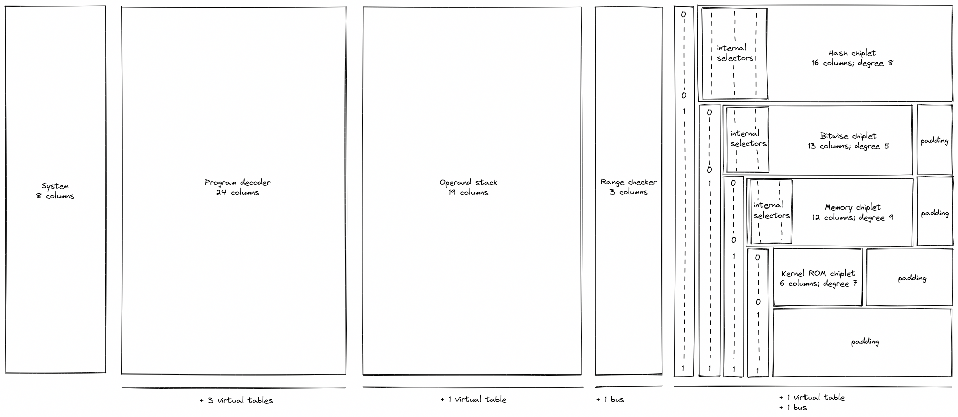
As can be seen from the above, the system, decoder, stack, and range checker components use dedicated sets of columns, while all chiplets share the same columns. To differentiate between chiplets, we use a set of binary selector columns, a combination of which uniquely identifies each chiplet.
The system component does not yet have a dedicated documentation section, since the design is likely to change. However, the following two columns are not expected to change:
clkwhich is used to keep track of the current VM cycle. Values in this column start out at and are incremented by with each cycle.fmpwhich contains the value of the free memory pointer used for specifying the region of memory available to procedure locals.
AIR constraints for the fmp column are described in system operations section. For the clk column, the constraints are straightforward:
Programs in Miden VM
Miden VM consumes programs in a form of a Merkelized Abstract Syntax Tree (MAST). This tree is a binary tree where each node is a code block. The VM starts execution at the root of the tree, and attempts to recursively execute each required block according to its semantics. If the execution of a code block fails, the VM halts at that point and no further blocks are executed. A set of currently available blocks and their execution semantics are described below.
Code blocks
Join block
A join block is used to describe sequential execution. When the VM encounters a join block, it executes its left child first, and then executes its right child.
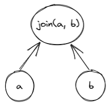
A join block must always have two children, and thus, cannot be a leaf node in the tree.
Split block
A split block is used to describe conditional execution. When the VM encounters a split block, it checks the top of the stack. If the top of the stack is , it executes the left child, if the top of the stack is , it executes the right child. If the top of the stack is neither nor , the execution fails.
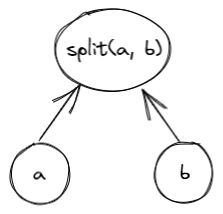
A split block must always have two children, and thus, cannot be a leaf node in the tree.
Loop block
A loop block is used to describe condition-based iterative execution. When the VM encounters a loop block, it checks the top of the stack. If the top of the stack is , it executes the loop body, if the top of the stack is , the block is not executed. If the top of the stack is neither nor , the execution fails.
After the body of the loop is executed, the VM checks the top of the stack again. If the top of the stack is , the body is executed again, if the top of the stack is , the loop is exited. If the top of the stack is neither nor , the execution fails.
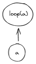
A loop block must always have one child, and thus, cannot be a leaf node in the tree.
Dyn block
A dyn block is used to describe a node whose target is specified dynamically via the stack. When the VM encounters a dyn block, it executes a program which hashes to the target specified by the top of the stack. Thus, it has a dynamic target rather than a hardcoded target. In order to execute a dyn block, the VM must be aware of a program with the hash value that is specified by the top of the stack. Otherwise, the execution fails.
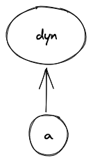
A dyn block must always have one (dynamically-specified) child. Thus, it cannot be a leaf node in the tree.
Call block
A call block is used to describe a function call which is executed in a user context. When the VM encounters a call block, it creates a new user context, then executes a program which hashes to the target specified by the call block in the new context. Thus, in order to execute a call block, the VM must be aware of a program with the specified hash. Otherwise, the execution fails. At the end of the call block, execution returns to the previous context.
When executing a call block, the VM does the following:
- Checks if a syscall is already being executed and fails if so.
- Sets the depth of the stack to 16.
- Upon return, checks that the depth of the stack is 16. If so, the original stack depth is restored. Otherwise, an error occurs.
A call block does not have any children. Thus, it must be leaf node in the tree.
Syscall block
A syscall block is used to describe a function call which is executed in the root context. When the VM encounters a syscall block, it returns to the root context, then executes a program which hashes to the target specified by the syscall block. Thus, in order to execute a syscall block, the VM must be aware of a program with the specified hash, and that program must belong to the kernel against which the code is compiled. Otherwise, the execution fails. At the end of the syscall block, execution returns to the previous context.
When executing a syscall block, the VM does the following:
- Checks if a syscall is already being executed and fails if so.
- Sets the depth of the stack to 16.
- Upon return, checks that the depth of the stack is 16. If so, the original stack depth is restored. Otherwise, an error occurs.
A syscall block does not have any children. Thus, it must be leaf node in the tree.
Span block
A span block is used to describe a linear sequence of operations. When the VM encounters a span block, it breaks the sequence of operations into batches and groups according to the following rules:
- A group is represented by a single field element. Thus, assuming a single operation can be encoded using 7 bits, and assuming we are using a 64-bit field, a single group may encode up to 9 operations or a single immediate value.
- A batch is a set of groups which can be absorbed by a hash function used by the VM in a single permutation. For example, assuming the hash function can absorb up to 8 field elements in a single permutation, a single batch may contain up to 8 groups.
- There is no limit on the number of batches contained within a single span.
Thus, for example, executing 8 pushes in a row will result in two operation batches as illustrated in the picture below:
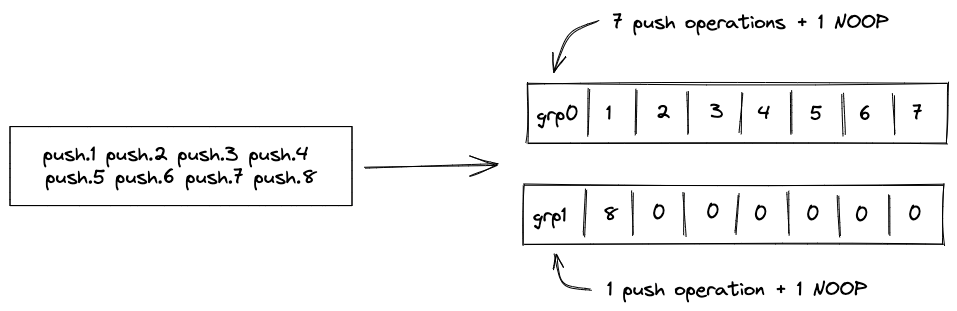
- The first batch will contain 8 groups, with the first group containing 7
PUSHopcodes and 1NOOP, and the remaining 7 groups containing immediate values for each of the push operations. The reason for theNOOPis explained later in this section. - The second batch will contain 2 groups, with the first group containing 1
PUSHopcode and 1NOOP, and the second group containing the immediate value for the last push operation.
If a sequence of operations does not have any operations which carry immediate values, up to 72 operations can fit into a single batch.
From the user's perspective, all operations are executed in order, however, the VM may insert occasional NOOPs to ensure proper alignment of all operations in the sequence. Currently, the alignment requirements are as follows:
- An operation carrying an immediate value cannot be the last operation in a group. Thus, for example, if a
PUSHoperation is the last operation in a group, the VM will insert aNOOPafter it.
A span block does not have any children, and thus, must be leaf node in the tree.
Program example
Consider the following program, where , etc. represent individual operations:
a_0, ..., a_i
if.true
    b_0, ..., b_j
else
    c_0, ..., c_k
    while.true
        d_0, ..., d_n
    end
    e_0, ..., e_m
end
f_0, ..., f_l
A MAST for this program would look as follows:
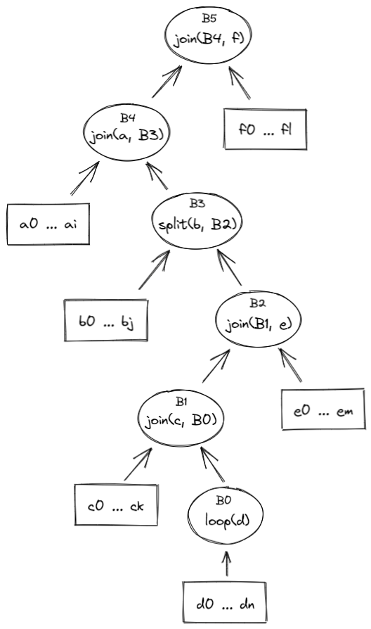
Execution of this program would proceed as follows:
- The VM will start execution at the root of the program which is block .
- Since, is a join block, the VM will attempt to execute block first, and only after that execute block .
- Block is also a join block, and thus, the VM will execute block by executing operations in sequence, and then execute block .
- Block is a split block, and thus, the VM will pop the value off the top of the stack. If the popped value is , operations from block will be executed in sequence. If the popped value is , then the VM will attempt to execute block .
- is a join block, thus, the VM will try to execute block first, and then execute operations from block .
- Block is also a join_block, and thus, the VM will first execute all operations in block , and then will attempt to execute block .
- Block is a loop block, thus, the VM will pop the value off the top of the stack. If the pooped value is , the VM will execute the body of the loop defined by block . If the popped value is , the VM will not execute block and instead will move up the tree executing first block , then .
- If the VM does enter the loop, then after operation is executed, the VM will pop the value off the top of the stack again. If the popped value is , the VM will execute block again, and again until the top of the stack becomes . Once the top of the stack becomes , the VM will exit the loop and will move up the tree executing first block , then .
Program hash computation
Every Miden VM program can be reduced to a unique hash value. Specifically, it is infeasible to find two Miden VM programs with distinct semantics which hash to the same value. Padding a program with NOOPs does not change a program's execution semantics, and thus, programs which differ only in the number and/or placement of NOOPs may hash to the same value, although in most cases padding with NOOP should not affect program hash.
To prevent program hash collisions we implement domain separation across the variants of control blocks. We define the domain value to be the opcode of the operation that initializes the control block.
Below we denote to be an arithmetization-friendly hash function with -element output and capable of absorbing elements in a single permutation. The hash domain is specified as the subscript of the hash function and its value is used to populate the second capacity register upon initialization of control block hashing - .
- The hash of a join block is computed as , where and are hashes of the code block being joined.
- The hash of a split block is computed as , where is a hash of a code block corresponding to the true branch of execution, and is a hash of a code block corresponding to the false branch of execution.
- The hash of a loop block is computed as , where is a hash of a code block corresponding to the loop body.
- The hash of a dyn block is set to a constant, so it is the same for all dyn blocks. It does not depend on the hash of the dynamic child. This constant is computed as the RPO hash of two empty words (
[ZERO, ZERO, ZERO, ZERO]) using a domain value ofDYN_DOMAIN, whereDYN_DOMAINis the op code of theDynoperation. - The hash of a call block is computed as , where is a hash of a program of which the VM is aware.
- The hash of a syscall block is computed as , where is a hash of a program belonging to the kernel against which the code was compiled.
- The hash of a span block is computed as , where is the th batch of operations in the span block. Each batch of operations is defined as containing field elements, and thus, hashing a -batch span block requires absorption steps.
- In cases when the number of operations is insufficient to fill the last batch entirely,
NOOPsare appended to the end of the last batch to ensure that the number of operations in the batch is always equal to .
- In cases when the number of operations is insufficient to fill the last batch entirely,
Miden VM Program decoder
Miden VM program decoder is responsible for ensuring that a program with a given MAST root is executed by the VM. As the VM executes a program, the decoder does the following:
- Decodes a sequence of field elements supplied by the prover into individual operation codes (or opcodes for short).
- Organizes the sequence of field elements into code blocks, and computes the hash of the program according to the methodology described here.
At the end of program execution, the decoder outputs the computed program hash. This hash binds the sequence of opcodes executed by the VM to a program the prover claims to have executed. The verifier uses this hash during the STARK proof verification process to verify that the proof attests to a correct execution of a specific program (i.e., the prover didn't claim to execute program while in fact executing a different program ).
The sections below describe how Miden VM decoder works. Throughout these sections we make the following assumptions:
- An opcode requires bits to represent.
- An immediate value requires one full field element to represent.
- A
NOOPoperation has a numeric value of , and thus, can be encoded as seven zeros. Executing aNOOPoperation does not change the state of the VM, but it does advance operation counter, and may affect program hash.
Program execution
Miden VM programs consist of a set of code blocks organized into a binary tree. The leaves of the tree contain linear sequences of instructions, and control flow is defined by the internal nodes of the tree.
Managing control flow in the VM is accomplished by executing control flow operations listed in the table below. Each of these operations requires exactly one VM cycle to execute.
| Operation | Description |
|---|---|
JOIN | Initiates processing of a new Join block. |
SPLIT | Initiates processing of a new Split block. |
LOOP | Initiates processing of a new Loop block. |
REPEAT | Initiates a new iteration of an executing loop. |
SPAN | Initiates processing of a new Span block. |
RESPAN | Initiates processing of a new operation batch within a span block. |
DYN | Initiates processing of a new Dyn block. |
CALL | Initiates processing of a new Call block. |
SYSCALL | Initiates processing ofa new Syscall block. |
END | Marks the end of a program block. |
HALT | Marks the end of the entire program. |
Let's consider a simple program below:
begin
    <operations1>
    if.true
        <operations2>
    else
        <operations3>
    end
end
Block structure of this program is shown below.
JOIN
    SPAN
        <operations1>
    END
    SPLIT
        SPAN
            <operations2>
        END
        SPAN
            <operations3>
        END
    END
END
Executing this program on the VM can result in one of two possible instruction sequences. First, if after operations in <operations1> are executed the top of the stack is , the VM will execute the following:
JOIN
SPAN
<operations1>
END
SPLIT
SPAN
<operations2>
END
END
END
HALT
However, if after <operations1> are executed, the top of the stack is , the VM will execute the following:
JOIN
SPAN
<operations1>
END
SPLIT
SPAN
<operations3>
END
END
END
HALT
The main task of the decoder is to output exactly the same program hash, regardless of which one of the two possible execution paths was taken. However, before we can describe how this is achieved, we need to give an overview of the overall decoder structure.
Decoder structure
The decoder is one of the more complex parts of the VM. It consists of the following components:
- Main execution trace consisting of trace columns which contain the state of the decoder at a given cycle of a computation.
- Connection to the hash chiplet, which is used to offload hash computations from the decoder.
- virtual tables (implemented via multi-set checks), which keep track of code blocks and operations executing on the VM.
Decoder trace
Decoder trace columns can be grouped into several logical sets of registers as illustrated below.

These registers have the following meanings:
- Block address register . This register contains address of the hasher for the current block (row index from the auxiliary hashing table). It also serves the role of unique block identifiers. This is convenient, because hasher addresses are guaranteed to be unique.
- Registers , which encode opcodes for operation to be executed by the VM. Each of these registers can contain a single binary value (either or ). And together these values describe a single opcode.
- Hasher registers . When control flow operations are executed, these registers are used to provide inputs for the current block's hash computation (e.g., for
JOIN,SPLIT,LOOP,SPAN,CALL,SYSCALLoperations) or to record the result of the hash computation (i.e., forENDoperation). However, when regular operations are executed, of these registers are used to help with op group decoding, and the remaining can be used to hold operation-specific helper variables. - Register which contains a binary flag indicating whether the VM is currently executing instructions inside a span block. The flag is set to when the VM executes non-control flow instructions, and is set to otherwise.
- Register which keeps track of the number of unprocessed operation groups in a given span block.
- Register which keeps track of a currently executing operation's index within its operation group.
- Operation batch flags which indicate how many operation groups a given operation batch contains. These flags are set only for
SPANandRESPANoperations, and are set to 's otherwise. - Two additional registers (not shown) are used primarily for constraint degree reduction.
Program block hashing
To compute hashes of program blocks, the decoder relies on the hash chiplet. Specifically, the decoder needs to perform two types of hashing operations:
- A simple 2-to-1 hash, where we provide a sequence of field elements, and get back field elements representing the result. Computing such a hash requires rows in the hash chiplet.
- A sequential hash of elements. Computing such a hash requires multiple absorption steps, and at each step field elements are absorbed into the hasher. Thus, computing a sequential hash of elements requires rows in the hash chiplet. At the end, we also get field elements representing the result.
To make hashing requests to the hash chiplet and to read the results from it, we will need to divide out relevant values from the chiplets bus column as described below.
Simple 2-to-1 hash
To initiate a 2-to-1 hash of elements () we need to divide by the following value:
where:
- is a label indicating beginning of a new permutation. Value of this label is computed based on hash chiplet selector flags according to the methodology described here.
- is the address of the row at which the hashing begins.
- Some values are skipped in the above (e.g., ) because of the specifics of how auxiliary hasher table rows are reduced to field elements (described here). For example, is used as a coefficient for node index values during Merkle path computations in the hasher, and thus, is not relevant in this case. The term is omitted when the number of items being hashed is a multiple of the rate width () because it is multiplied by 0 - the value of the first capacity register as determined by the hasher chiplet logic.
To read the -element result (), we need to divide by the following value:
where:
- is a label indicating return of the hash value. Value of this label is computed based on hash chiplet selector flags according to the methodology described here.
- is the address of the row at which the hashing began.
Sequential hash
To initiate a sequential hash of elements (), we need to divide by the following value:
This also absorbs the first elements of the sequence into the hasher state. Then, to absorb the next sequence of elements (e.g., ), we need to divide by the following value:
Where is a label indicating absorption of more elements into the hasher state. Value of this label is computed based on hash chiplet selector flags according to the methodology described here.
We can keep absorbing elements into the hasher in the similar manner until all elements have been absorbed. Then, to read the result (e.g., ), we need to divide by the following value:
Thus, for example, if , the result will of the hash will be available at hasher row .
Control flow tables
In addition to the hash chiplet, control flow operations rely on virtual tables: block stack table, block hash table, and op group table. These tables are virtual in that they don't require separate trace columns. Their state is described solely by running product columns: , , and . The tables are described in the following sections.
Block stack table
When the VM starts executing a new program block, it adds its block ID together with the ID of its parent block (and some additional info) to the block stack table. When a program block is fully executed, it is removed from the table. In this way, the table represents a stack of blocks which are currently executing on the VM. By the time program execution completes, block stack table must be empty.
The block stack table is also used to ensure that execution contexts are managed properly across the CALL and SYSCALL operations.
The table can be thought of as consisting of columns as shown below:
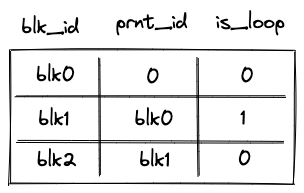
where:
- The first column () contains the ID of the block.
- The second column () contains the ID of the parent block. If the block has no parent (i.e., it is a root block of the program), parent ID is 0.
- The third column () contains a binary value which is set to is the block is a loop block, and to otherwise.
- The following 8 columns are only set to non-zero values for
CALLandSYSCALLoperations. They save all the necessary information to be able to restore the parent context properly upon the correspondingENDoperation- the
prnt_b0andprnt_b1columns refer to the stack helper columns B0 and B1 (current stack depth and last overflow address, respectively)
- the
In the above diagram, the first 2 rows correspond to 2 different CALL operations. The first CALL operation is called from the root context, and hence its parent fn hash is the zero hash. Additionally, the second CALL operation has a parent fn hash of [h0, h1, h2, h3], indicating that the first CALL was to a procedure with that hash.
Running product column is used to keep track of the state of the table. At any step of the computation, the current value of defines which rows are present in the table.
To reduce a row in the block stack table to a single value, we compute the following.
where are the random values provided by the verifier.
Block hash table
When the VM starts executing a new program block, it adds hashes of the block's children to the block hash table. And when the VM finishes executing a block, it removes its hash from the block hash table. Thus, by the time program execution completes, block hash table must be empty.
The table can be thought of as consisting of columns as shown below:
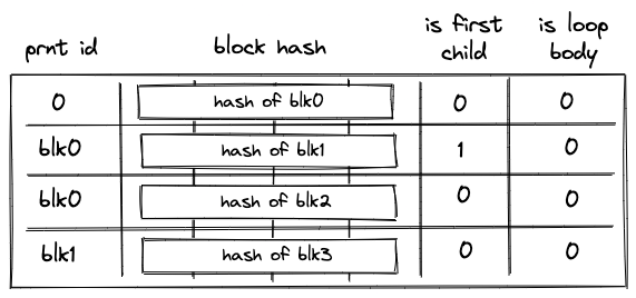
where:
- The first column () contains the ID of the block's parent. For program root, parent ID is .
- The next columns () contain the hash of the block.
- The next column () contains a binary value which is set to if the block is the first child of a join block, and to otherwise.
- The last column () contains a binary value which is set to if the block is a body of a loop, and to otherwise.
Running product column is used to keep track of the state of the table. At any step of the computation, the current value of defines which rows are present in the table.
To reduce a row in the block hash table to a single value, we compute the following.
Where are the random values provided by the verifier.
Unlike other virtual tables, block hash table does not start out in an empty state. Specifically, it is initialized with a single row containing the hash of the program's root block. This needs to be done because the root block does not have a parent and, thus, otherwise it would never be added to the block hash table.
Initialization of the block hash table is done by setting the initial value of to the value of the row containing the hash of a program's root block.
Op group table
Op group table is used in decoding of span blocks, which are leaves in a program's MAST. As described here, a span block can contain one or more operation batches, each batch containing up to operation groups.
When the VM starts executing a new batch of operations, it adds all operation groups within a batch, except for the first one, to the op group table. Then, as the VM starts executing an operation group, it removes the group from the table. Thus, by the time all operation groups in a batch have been executed, the op group table must be empty.
The table can be thought of as consisting of columns as shown below:
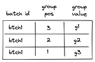
The meaning of the columns is as follows:
- The first column () contains operation batch ID. During the execution of the program, each operation batch is assigned a unique ID.
- The second column () contains the position of the group in the span block (not just in the current batch). The position is -based and is counted from the end. Thus, for example, if a span block consists of a single batch with groups, the position of the first group would be , the position of the second group would be etc. (the reason for this is explained in this section). Note that the group with position is not added to the table, because it is the first group in the batch, so the first row of the table will be for the group with position .
- The third column () contains the actual values of operation groups (this could include up to opcodes or a single immediate value).
Permutation column is used to keep track of the state of the table. At any step of the computation, the current value of defines which rows are present in the table.
To reduce a row in the op group table to a single value, we compute the following.
Where are the random values provided by the verifier.
Control flow operation semantics
In this section we describe high-level semantics of executing all control flow operations. The descriptions are not meant to be complete and omit some low-level details. However, they provide good intuition on how these operations work.
JOIN operation
Before a JOIN operation is executed by the VM, the prover populates registers with hashes of left and right children of the join program block as shown in the diagram below.
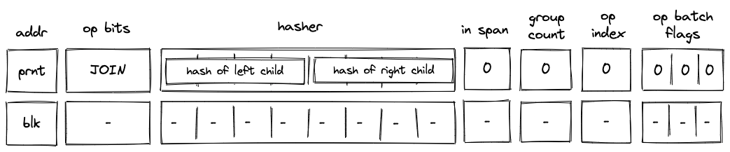
In the above diagram, blk is the ID of the join block which is about to be executed. blk is also the address of the hasher row in the auxiliary hasher table. prnt is the ID of the block's parent.
When the VM executes a JOIN operation, it does the following:
- Adds a tuple
(blk, prnt, 0, 0...)to the block stack table. - Adds tuples
(blk, left_child_hash, 1, 0)and(blk, right_child_hash, 0, 0)to the block hash table. - Initiates a 2-to-1 hash computation in the hash chiplet (as described here) using
blkas row address in the auxiliary hashing table and as input values.
SPLIT operation
Before a SPLIT operation is executed by the VM, the prover populates registers with hashes of true and false branches of the split program block as shown in the diagram below.
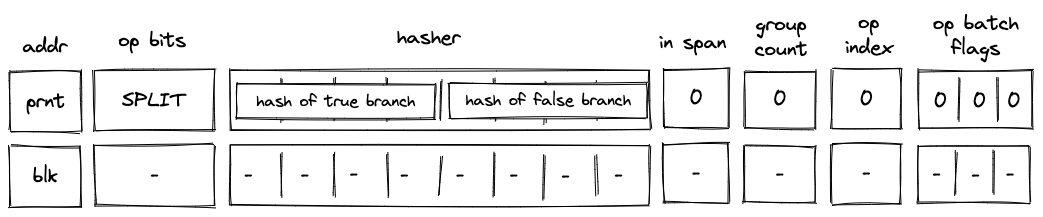
In the above diagram, blk is the ID of the split block which is about to be executed. blk is also the address of the hasher row in the auxiliary hasher table. prnt is the ID of the block's parent.
When the VM executes a SPLIT operation, it does the following:
- Adds a tuple
(blk, prnt, 0, 0...)to the block stack table. - Pops the stack and:
a. If the popped value is , adds a tuple(blk, true_branch_hash, 0, 0)to the block hash table.
b. If the popped value is , adds a tuple(blk, false_branch_hash, 0, 0)to the block hash table.
c. If the popped value is neither nor , the execution fails. - Initiates a 2-to-1 hash computation in the hash chiplet (as described here) using
blkas row address in the auxiliary hashing table and as input values.
LOOP operation
Before a LOOP operation is executed by the VM, the prover populates registers with hash of the loop's body as shown in the diagram below.
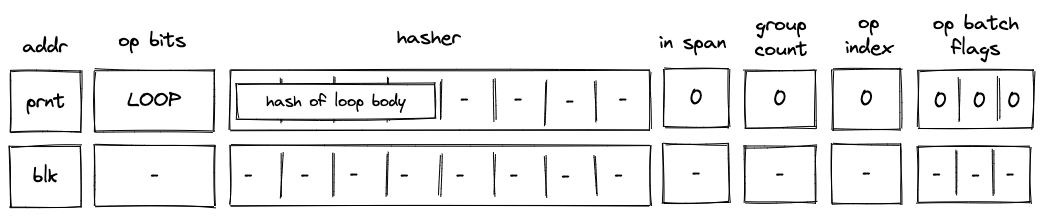
In the above diagram, blk is the ID of the loop block which is about to be executed. blk is also the address of the hasher row in the auxiliary hasher table. prnt is the ID of the block's parent.
When the VM executes a LOOP operation, it does the following:
- Pops the stack and:
a. If the popped value is adds a tuple(blk, prnt, 1, 0...)to the block stack table (the1indicates that the loop's body is expected to be executed). Then, adds a tuple(blk, loop_body_hash, 0, 1)to the block hash table.
b. If the popped value is , adds(blk, prnt, 0, 0...)to the block stack table. In this case, nothing is added to the block hash table.
c. If the popped value is neither nor , the execution fails. - Initiates a 2-to-1 hash computation in the hash chiplet (as described here) using
blkas row address in the auxiliary hashing table and as input values.
SPAN operation
Before a SPAN operation is executed by the VM, the prover populates registers with contents of the first operation batch of the span block as shown in the diagram below. The prover also sets the group count register to the total number of operation groups in the span block.
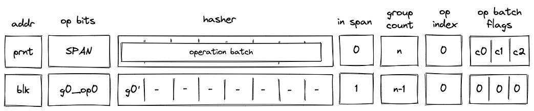
In the above diagram, blk is the ID of the span block which is about to be executed. blk is also the address of the hasher row in the auxiliary hasher table. prnt is the ID of the block's parent. g0_op0 is the first operation of the batch, and g_0' is the first operation group of the batch with the first operation removed.
When the VM executes a SPAN operation, it does the following:
- Adds a tuple
(blk, prnt, 0, 0...)to the block stack table. - Adds groups of the operation batch, as specified by op batch flags (see here) to the op group table.
- Initiates a sequential hash computation in the hash chiplet (as described here) using
blkas row address in the auxiliary hashing table and as input values. - Sets the
in_spanregister to . - Decrements
group_countregister by . - Sets the
op_indexregister to .
DYN operation
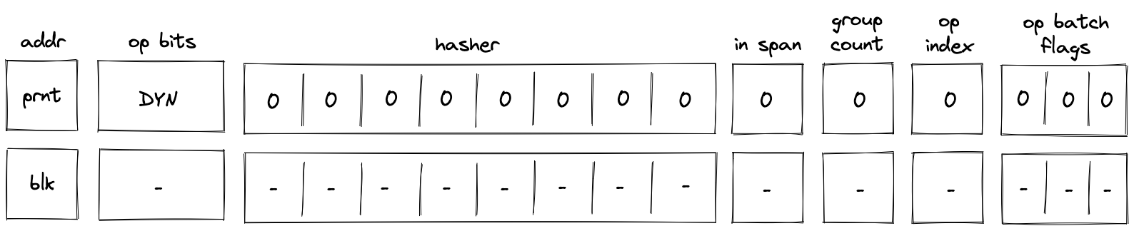
In the above diagram, blk is the ID of the dyn block which is about to be executed. blk is also the address of the hasher row in the auxiliary hasher table. p_addr is the ID of the block's parent.
When the VM executes a DYN operation, it does the following:
- Adds a tuple
(blk, p_addr, 0, 0...)to the block stack table. - Sends a memory read request to the memory chiplet, using
s0as the memory address. The resulthash of calleeis placed in the decoder hasher trace at . - Adds the tuple
(blk, hash of callee, 0, 0)to the block hash table. - Initiates a 2-to-1 hash computation in the hash chiplet (as described here) using
blkas row address in the auxiliary hashing table and[ZERO; 8]as input values. - Performs a stack left shift
- Above
s16was pulled from the stack overflow table if present; otherwise set to0.
- Above
Note that unlike DYNCALL, the fmp, ctx, in_syscall and fn_hash registers are unchanged.
DYNCALL operation
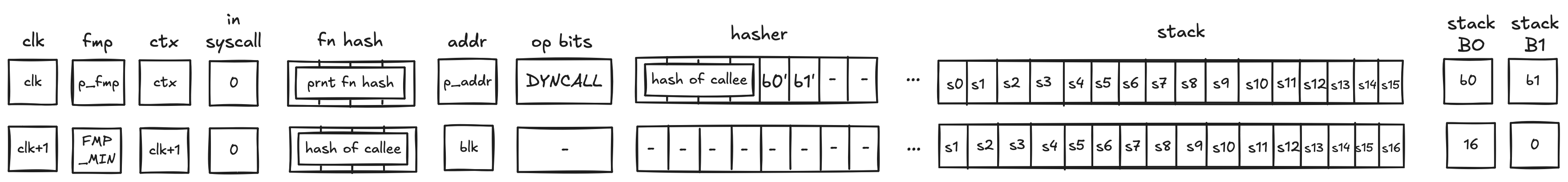
In the above diagram, blk is the ID of the dyn block which is about to be executed. blk is also the address of the hasher row in the auxiliary hasher table. p_addr is the ID of the block's parent.
When the VM executes a DYNCALL operation, it does the following:
- Adds a tuple
(blk, p_addr, 0, ctx, fmp, b_0, b_1, fn_hash[0..3])to the block stack table. - Sends a memory read request to the memory chiplet, using
s0as the memory address. The resulthash of calleeis placed in the decoder hasher trace at . - Adds the tuple
(blk, hash of callee, 0, 0)to the block hash table. - Initiates a 2-to-1 hash computation in the hash chiplet (as described here) using
blkas row address in the auxiliary hashing table and[ZERO; 8]as input values. - Performs a stack left shift
- Above
s16was pulled from the stack overflow table if present; otherwise set to0.
- Above
Similar to CALL, DYNCALL resets the fmp, sets up a new ctx, and sets the fn_hash registers to the callee hash. in_syscall needs to be 0, since calls are not allowed during a syscall.
END operation
Before an END operation is executed by the VM, the prover populates registers with the hash of the block which is about to end. The prover also sets values in and registers as follows:
- is set to if the block is a body of a loop block. We denote this value as
f0. - is set to if the block is a loop block. We denote this value as
f1. - is set to if the block is a call block. We denote this value as
f2. - is set to if the block is a syscall block. We denote this value as
f3.
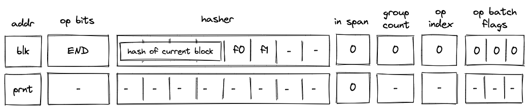
In the above diagram, blk is the ID of the block which is about to finish executing. prnt is the ID of the block's parent.
When the VM executes an END operation, it does the following:
- Removes a tuple from the block stack table.
- if
f2orf3is set, we remove a row(blk, prnt, 0, ctx_next, fmp_next, b0_next, b1_next, fn_hash_next[0..4])- in the above, the
x_nextvariables denote the columnxin the next row
- in the above, the
- else, we remove a row
(blk, prnt, f1, 0, 0, 0, 0, 0)
- if
- Removes a tuple
(prnt, current_block_hash, nxt, f0)from the block hash table, where if the next operation is eitherENDorREPEAT, and otherwise. - Reads the hash result from the hash chiplet (as described here) using
blk + 7as row address in the auxiliary hashing table. - If (i.e., we are exiting a loop block), pops the value off the top of the stack and verifies that the value is .
- Verifies that
group_countregister is set to .
HALT operation
Before a HALT operation is executed by the VM, the VM copies values in registers to the next row as illustrated in the diagram below:
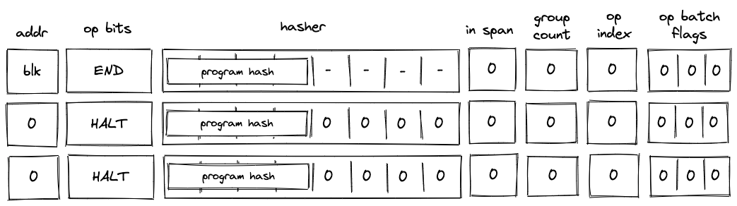
In the above diagram, blk is the ID of the block which is about to finish executing.
When the VM executes a HALT operation, it does the following:
- Verifies that block address register is set to .
- If we are not at the last row of the trace, verifies that the next operation is
HALT. - Copies values of registers to the next row.
- Populates all other decoder registers with 's in the next row.
REPEAT operation
Before a REPEAT operation is executed by the VM, the VM copies values in registers to the next row as shown in the diagram below.
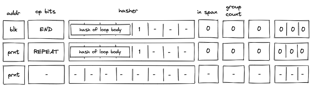
In the above diagram, blk is the ID of the loop's body and prnt is the ID of the loop.
When the VM executes a REPEAT operation, it does the following:
- Checks whether register is set to . If it isn't (i.e., we are not in a loop), the execution fails.
- Pops the stack and if the popped value is , adds a tuple
(prnt, loop_body_loop 0, 1)to the block hash table. If the popped value is not , the execution fails.
The effect of the above is that the VM needs to execute the loop's body again to clear the block hash table.
RESPAN operation
Before a RESPAN operation is executed by the VM, the VM copies the ID of the current block blk and the number of remaining operation groups in the span to the next row, and sets the value of in_span column to . The prover also sets the value of register for the next row to the ID of the current block's parent prnt as shown in the diagram below:
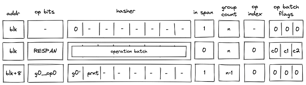
In the above diagram, g0_op0 is the first operation of the new operation batch, and g0' is the first operation group of the batch with g0_op0 operation removed.
When the VM executes a RESPAN operation, it does the following:
- Increments block address by .
- Removes the tuple
(blk, prnt, 0, 0...)from the block stack table. - Adds the tuple
(blk+8, prnt, 0, 0...)to the block stack table. - Absorbs values in registers into the hasher state of the hash chiplet (as described here).
- Sets the
in_spanregister to . - Adds groups of the operation batch, as specified by op batch flags (see here) to the op group table using
blk+8as batch ID.
The net result of the above is that we incremented the ID of the current block by and added the next set of operation groups to the op group table.
CALL operation
Recall that the purpose of a CALL operation is to execute a procedure in a new execution context. Specifically, this means that the entire memory is zero'd in the new execution context, and the stack is truncated to a depth of 16 (i.e. any element in the stack overflow table is not available in the new context). On the corresponding END instruction, the prover will restore the previous execution context (verified by the block stack table).
Before a CALL operation, the prover populates registers with the hash of the procedure being called. In the next row, the prover
- resets the FMP register (free memory pointer),
- sets the context ID to the next row's CLK value
- sets the
fn hashregisters to the hash of the callee- This register is what the
callerinstruction uses to return the hash of the caller in a syscall
- This register is what the
- resets the stack
B0register to 16 (which tracks the current stack depth) - resets the overflow address to 0 (which tracks the "address" of the last element added to the overflow table)
- it is set to 0 to indicate that the overflow table is empty
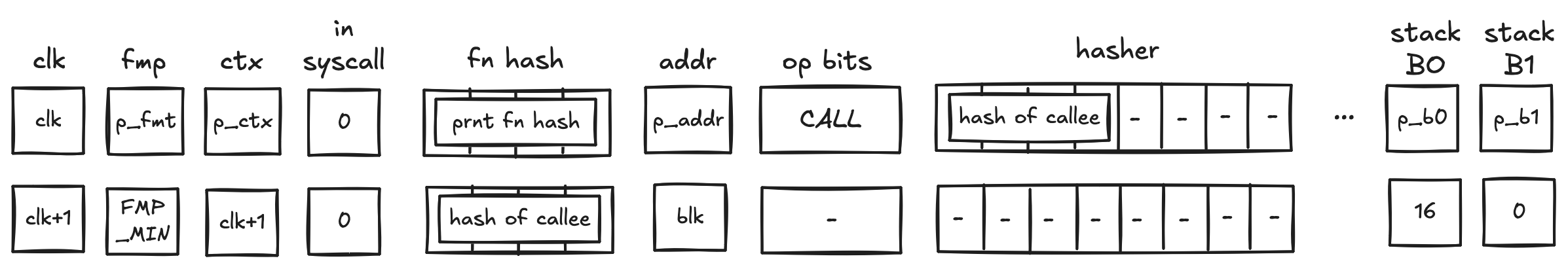
In the above diagram, blk is the ID of the call block which is about to be executed. blk is also the address of the hasher row in the auxiliary hasher table. prnt is the ID of the block's parent.
When the VM executes a CALL operation, it does the following:
- Adds a tuple
(blk, prnt, 0, p_ctx, p_fmp, p_b0, p_b1, prnt_fn_hash[0..4])to the block stack table. - Initiates a 2-to-1 hash computation in the hash chiplet (as described here) using
blkas row address in the auxiliary hashing table and as input values.
SYSCALL operation
Similarly to the CALL operation, a SYSCALL changes the execution context. However, it always jumps back to the root context, and executes kernel procedures only.
Before a SYSCALL operation, the prover populates registers with the hash of the procedure being called. In the next row, the prover
- resets the FMP register (free memory pointer),
- sets the context ID to 0,
- does NOT modify the
fn hashregister- Hence, the
fn hashregister contains the procedure hash of the caller, to be accessed by thecallerinstruction,
- Hence, the
- resets the stack
B0register to 16 (which tracks the current stack depth) - resets the overflow address to 0 (which tracks the "address" of the last element added to the overflow table)
- it is set to 0 to indicate that the overflow table is empty
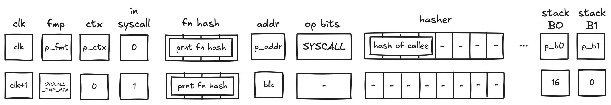
In the above diagram, blk is the ID of the syscall block which is about to be executed. blk is also the address of the hasher row in the auxiliary hasher table. prnt is the ID of the block's parent.
When the VM executes a SYSCALL operation, it does the following:
- Adds a tuple
(blk, prnt, 0, p_ctx, p_fmp, p_b0, p_b1, prnt_fn_hash[0..4])to the block stack table. - Sends a request to the kernel ROM chiplet indicating that
hash of calleeis being accessed.- this results in a fault if
hash of calleedoes not correspond to the hash of a kernel procedure
- this results in a fault if
- Initiates a 2-to-1 hash computation in the hash chiplet (as described here) using
blkas row address in the auxiliary hashing table and as input values.
Program decoding
When decoding a program, we start at the root block of the program. We can compute the hash of the root block directly from hashes of its children. The prover provides hashes of the child blocks non-deterministically, and we use them to compute the program's hash (here we rely on the hash chiplet). We then verify the program hash via boundary constraints. Thus, if the prover provided valid hashes for the child blocks, we will get the expected program hash.
Now, we need to verify that the VM executed the child blocks correctly. We do this recursively similar to what is described above: for each of the blocks, the prover provides hashes of its children non-deterministically and we verify that the hash has been computed correctly. We do this until we get to the leaf nodes (i.e., span blocks). Hashes of span blocks are computed sequentially from the instructions executed by the VM.
The sections below illustrate how different types of code blocks are decoded by the VM.
JOIN block decoding
When decoding a join bock, the VM first executes a JOIN operation, then executes the first child block, followed by the second child block. Once the children of the join block are executed, the VM executes an END operation. This is illustrated in the diagram below.
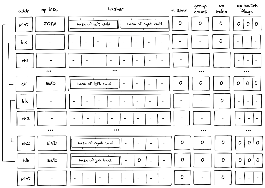
As described previously, when the VM executes a JOIN operation, hashes of both children are added to the block hash table. These hashes are removed only when the END operations for the child blocks are executed. Thus, until both child blocks are executed, the block hash table is not cleared.
SPLIT block decoding
When decoding a split block, the decoder pops an element off the top of the stack, and if the popped element is , executes the block corresponding to the true branch. If the popped element is , the decoder executes the block corresponding to the false branch. This is illustrated on the diagram below.
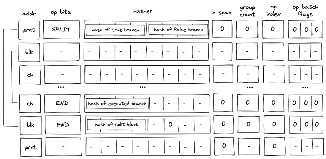
As described previously, when the VM executes a SPLIT operation, only the hash of the branch to be executed is added to the block hash table. Thus, until the child block corresponding to the required branch is executed, the block hash table is not cleared.
LOOP block decoding
When decoding a loop bock, we need to consider two possible scenarios:
- When the top of the stack is , we need to enter the loop and execute loop body at least once.
- When the top of the stack is, we need to skip the loop.
In both cases, we need to pop an element off the top of the stack.
Executing the loop
If the top of the stack is , the VM executes a LOOP operation. This removes the top element from the stack and adds the hash of the loop's body to the block hash table. It also adds a row to the block stack table setting the is_loop value to .
To clear the block hash table, the VM needs to execute the loop body (executing the END operation for the loop body block will remove the corresponding row from the block hash table). After loop body is executed, if the top of the stack is , the VM executes a REPEAT operation (executing REPEAT operation when the top of the stack is will result in an error). This operation again adds the hash of the loop's body to the block hash table. Thus, the VM needs to execute the loop body again to clear the block hash table.
This process is illustrated on the diagram below.
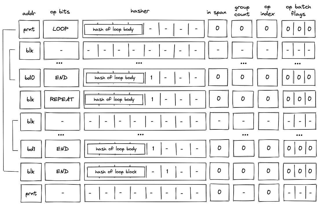
The above steps are repeated until the top of the stack becomes , at which point the VM executes the END operation. Since in the beginning we set is_loop column in the block stack table to , column will be set to when the END operation is executed. Thus, executing the END operation will also remove the top value from the stack. If the removed value is not , the operation will fail. Thus, the VM can exit the loop block only when the top of the stack is .
Skipping the loop
If the top of the stack is , the VM still executes the LOOP operation. But unlike in the case when we need to enter the loop, the VM sets is_loop flag to in the block stack table, and does not add any rows to the block hash table. The last point means that the only possible operation to be executed after the LOOP operation is the END operation. This is illustrated in the diagram below.
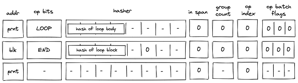
Moreover, since we've set the is_loop flag to , executing the END operation does not remove any items from the stack.
DYN block decoding
When decoding a dyn bock, the VM first executes a DYN operation, then executes the child block dynamically specified by the top of the stack. Once the child of the dyn block has been executed, the VM executes an END operation. This is illustrated in the diagram below.
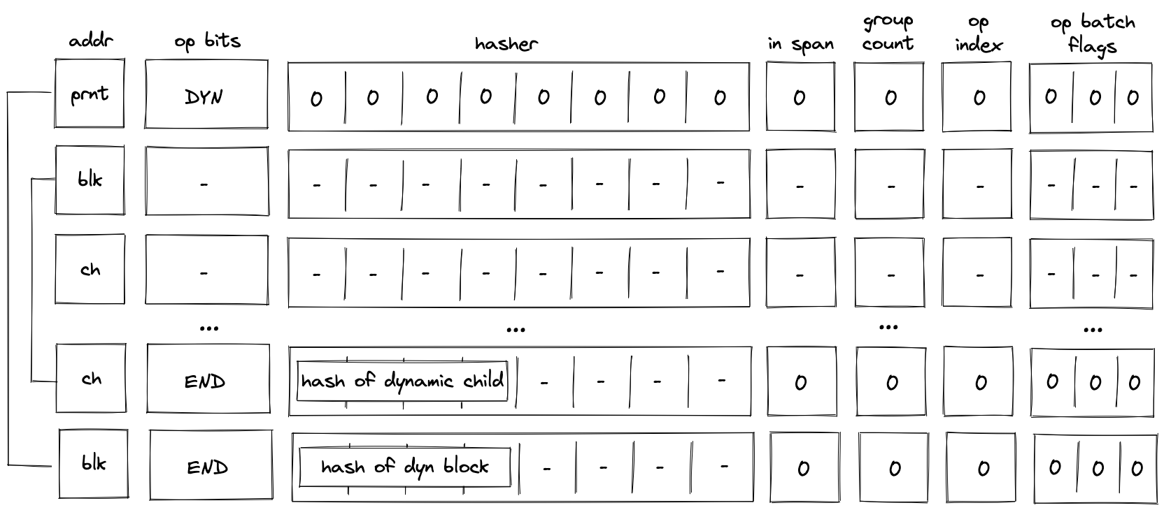
As described previously, when the VM executes a DYN operation, the hash of the child is added to the block hash table. This hash is removed only when the END operation for the child block is executed. Thus, until the child block corresponding to the dynamically specified target is executed, the block hash table is not cleared.
SPAN block decoding
As described here, a span block can contain one or more operation batches, each batch containing up to operation groups. At the high level, decoding of a span block is done as follows:
- At the beginning of the block, we make a request to the hash chiplet which initiates the hasher, absorbs the first operation batch ( field elements) into the hasher, and returns the row address of the hasher, which we use as the unique ID for the span block (see here).
- We then add groups of the operation batch, as specified by op batch flags (but always skipping the first one) to the op group table.
- We then remove operation groups from the op group table in the FIFO order one by one, and decode them in the manner similar to the one described here.
- Once all operation groups in a batch have been decoded, we absorb the next batch into the hasher and repeat the process described above.
- Once all batches have been decoded, we return the hash of the span block from the hasher.
Overall, three control flow operations are used when decoding a span block:
SPANoperation is used to initialize a hasher and absorbs the first operation batch into it.RESPANoperation is used to absorb any additional batches in the span block.ENDoperation is used to end the decoding of a span block and retrieve its hash from the hash chiplet.
Operation group decoding
As described here, an operation group is a sequence of operations which can be encoded into a single field element. For a field element of bits, we can fit up to operations into a group. We do this by concatenating binary representations of opcodes together with the first operation located in the least significant position.
We can read opcodes from the group by simply subtracting them from the op group value and then dividing the result by . Once the value of the op group reaches , we know that all opcodes have been read. Graphically, this can be illustrated like so:
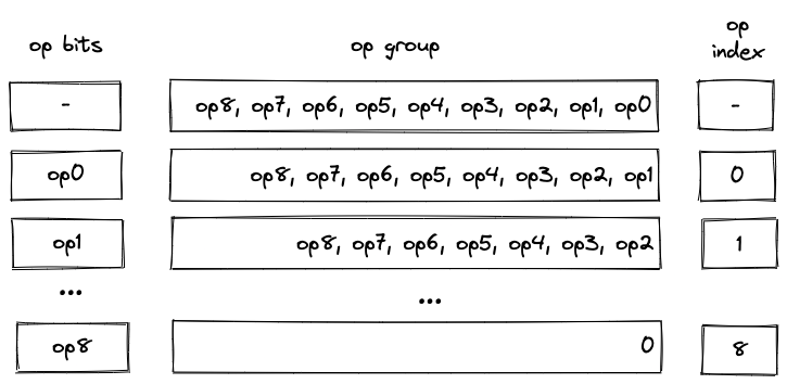
Notice that despite their appearance, op bits is actually separate registers, while op group is just a single register.
We also need to make sure that at most operations are executed as a part of a single group. For this purpose we use the op_index column. Values in this column start out at for each operation group, and are incremented by for each executed operation. To make sure that at most operations can be executed in a group, the value of the op_index column is not allowed to exceed .
Operation batch flags
Operation batch flags are used to specify how many operation groups comprise a given operation batch. For most batches, the number of groups will be equal to . However, for the last batch in a block (or for the first batch, if the block consists of only a single batch), the number of groups may be less than . Since processing of new batches starts only on SPAN and RESPAN operations, only for these operations the flags can be set to non-zero values.
To simplify the constraint system, the number of groups in a batch can be only one of the following values: , , , and . If the number of groups in a batch does not match one of these values, the batch is simply padded with NOOP's (one NOOP per added group). Consider the diagram below.
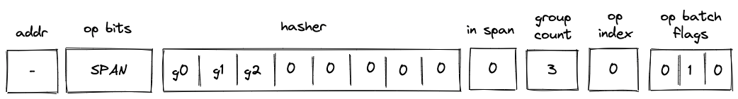
In the above, the batch contains operation groups. To bring the count up to , we consider the -th group (i.e., ) to be a part of the batch. Since a numeric value for NOOP operation is , op group value of can be interpreted as a single NOOP.
Operation batch flags (denoted as ), encode the number of groups and define how many groups are added to the op group table as follows:
(1, -, -)- groups. Groups in are added to the op group table.(0, 1, 0)- groups. Groups in are added to the op group table(0, 0, 1)- groups. Groups in is added to the op group table.(0, 1, 1)- group. Nothing is added to the op group table(0, 0, 0)- not aSPANorRESPANoperation.
Single-batch span
The simplest example of a span block is a block with a single batch. This batch may contain up to operation groups (e.g., ). Decoding of such a block is illustrated in the diagram below.
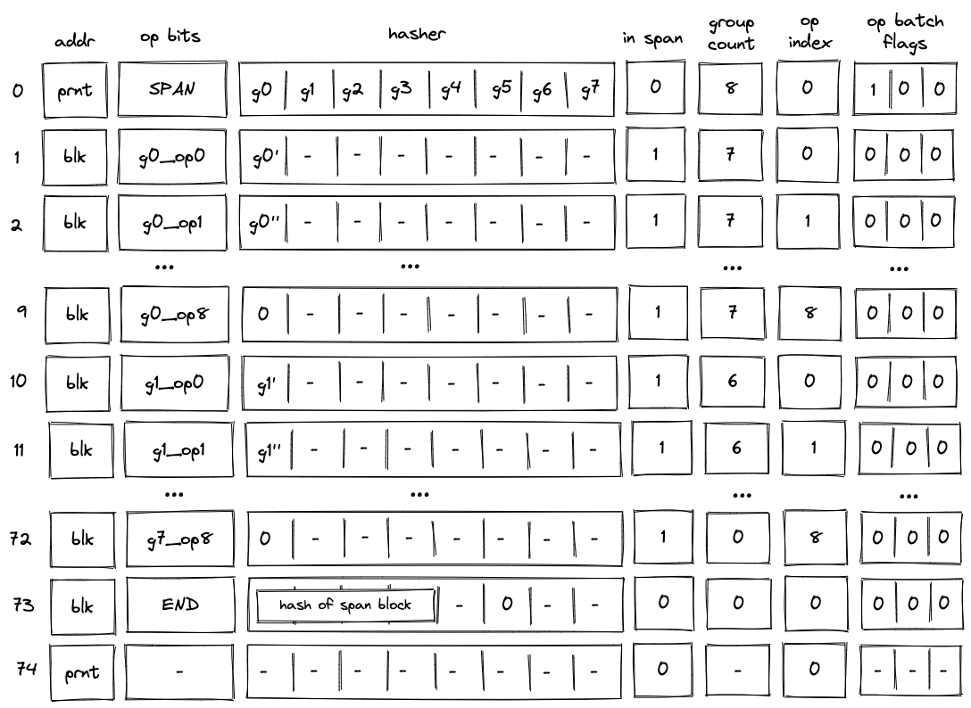
Before the VM starts processing this span block, the prover populates registers with operation groups . The prover also puts the total number of groups into the group_count register . In this case, the total number of groups is .
When the VM executes a SPAN operation, it does the following:
- Initiates hashing of elements using hash chiplet. The hasher address is used as the block ID
blk, and it is inserted intoaddrregister in the next row. - Adds a tuple
(blk, prnt, 0)to the block stack table. - Sets the
is_spanregister to in the next row. - Sets the
op_indexregister to in the next row. - Decrements
group_countregister by . - Sets
op bitsregisters at the next step to the first operation of , and also copies with the first operation removed (denoted as ) to the next row. - Adds groups to the op group table. Thus, after the
SPANoperation is executed, op group table looks as shown below.
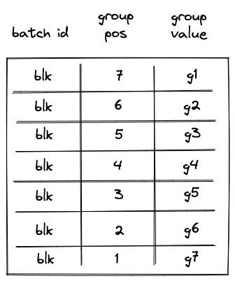
Then, with every step the next operation is removed from , and by step , the value of is . Once this happens, the VM does the following:
- Decrements
group_countregister by . - Sets
op bitsregisters at the next step to the first operation of . - Sets
hasherregister to the value of with the first operation removed (denoted as ). - Removes row
(blk, 7, g1)from the op group table. This row can be obtained by taking values from registers:addr,group_count, and for , where and refer to values in the next row for the first hasher column andop_bitscolumns respectively.
Note that we rely on the group_count column to construct the row to be removed from the op group table. Since group count is decremented from the total number of groups to , to remove groups from the op group table in correct order, we need to assign group position to groups in the op group table in the reverse order. For example, the first group to be removed should have position , the second group to be removed should have position etc.
Decoding of is performed in the same manner as decoding of : with every subsequent step the next operation is removed from until its value reaches , at which point, decoding of group begins.
The above steps are executed until value of group_count reaches . Once group_count reaches and the last operation group is executed, the VM executes the END operation. Semantics of the END operation are described here.
Notice that by the time we get to the END operation, all rows are removed from the op group table.
Multi-batch span
A span block may contain an unlimited number of operation batches. As mentioned previously, to absorb a new batch into the hasher, the VM executes a RESPAN operation. The diagram below illustrates decoding of a span block consisting of two operation batches.
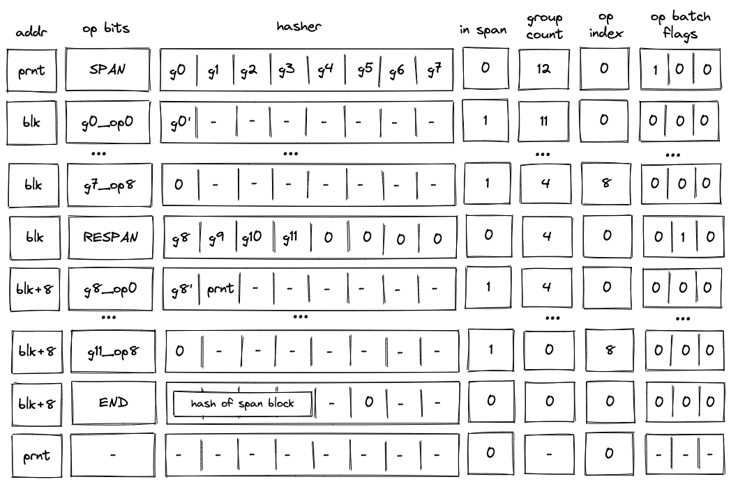
Decoding of such a block will look very similar to decoding of the single-span block described previously, but there also will be some differences.
First, after the SPAN operation is executed, the op group table will look as follows:
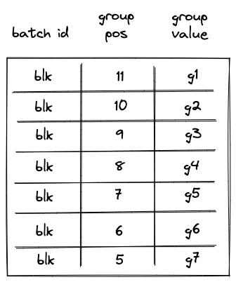
Notice that while the same groups () are added to the table, their positions now reflect the total number of groups in the span block.
Second, executing a RESPAN operation increments hasher address by . This is done because absorbing additional elements into the hasher state requires more rows in the auxiliary hasher table.
Incrementing value of addr register actually changes the ID of the span block (though, for a span block, it may be more appropriate to view values in this column as IDs of individual operation batches). This means that we also need to update the block stack table. Specifically, we need to remove row (blk, prnt, 0) from it, and replace it with row (blk + 8, prnt, 0). To perform this operation, the prover sets the value of in the next row to prnt.
Executing a RESPAN operation also adds groups to the op group table, which now would look as follows:
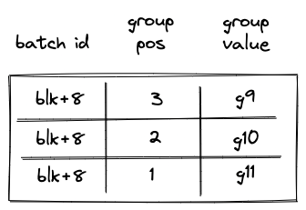
Then, the execution of the second batch proceeds in a manner similar to the first batch: we remove operations from the current op group, execute them, and when the value of the op group reaches , we start executing the next group in the batch. Thus, by the time we get to the END operation, the op group table should be empty.
When executing the END operation, the hash of the span block will be read from hasher row at address addr + 7, which, in our example, will be equal to blk + 15.
Handling immediate values
Miden VM operations can carry immediate values. Currently, the only such operation is a PUSH operation. Since immediate values can be thought of as constants embedded into program code, we need to make sure that changing immediate values affects program hash.
To achieve this, we treat immediate values in a manner similar to how we treat operation groups. Specifically, when computing hash of a span block, immediate values are absorbed into the hasher state in the same way as operation groups are. As mentioned previously, an immediate value is represented by a single field element, and thus, an immediate value takes place of a single operation group.
The diagram below illustrates decoding of a span block with operations one of which is a PUSH operation.
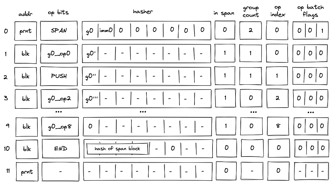
In the above, when the SPAN operation is executed, immediate value imm0 will be added to the op group table, which will look as follows:
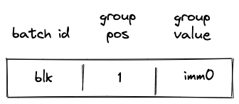
Then, when the PUSH operation is executed, the VM will do the following:
- Decrement
group_countby . - Remove a row from the op group table equal to
(addr, group_count, s0'), where is the value of the top of the stack at the next row (i.e., it is the value that is pushed onto the stack).
Thus, after the PUSH operation is executed, the op group table is cleared, and group count decreases to (which means that there are no more op groups to execute). Decoding of the rest of the op group proceeds as described in the previous sections.
Program decoding example
Let's run through an example of decoding a simple program shown previously:
begin
    <operations1>
    if.true
        <operations2>
    else
        <operations3>
    end
end
Translating this into code blocks with IDs assigned, we get the following:
b0: JOIN
    b1: SPAN
        <operations1>
    b1: END
    b2: SPLIT
        b3: SPAN
            <operations2>
        b3: END
        b4: SPAN
            <operations3>
        b4: END
    b2: END
b0: END
The root of the program is a join block . This block contains two children: a span bock and a split block . In turn, the split block contains two children: a span block and a span block .
When this program is executed on the VM, the following happens:
- Before the program starts executing, block hash table is initialized with a single row containing the hash of .
- Then,
JOINoperation for is executed. It adds hashes of and to the block hash table. It also adds an entry for to the block stack table. States of both tables after this step are illustrated below. - Then, span is executed and a sequential hash of its operations is computed. Also, when
SPANoperation for is executed, an entry for is added to the block stack table. At the end of (whenENDis executed), entries for are removed from both the block hash and block stack tables. - Then,
SPLIToperation for is executed. It adds an entry for to the block stack table. Also, depending on whether the top of the stack is or , either hash of or hash of is added to the block hash table. Let's say the top of the stack is . Then, at this point, the block hash and block stack tables will look like in the second picture below. - Then, span is executed and a sequential hash of its instructions is computed. Also, when
SPANoperation for is executed, an entry for is added to the block stack table. At the end of (whenENDis executed), entries for are removed from both the block hash and block stack tables. - Then,
ENDoperation for is executed. It removes the hash of from the block hash table, and also removes the entry for from the block stack table. The third picture below illustrates the states of block stack and block hash tables after this step. - Then,
ENDfor is executed, which removes entries for from the block stack and block hash tables. At this point both tables are empty. - Finally, a sequence of
HALToperations is executed until the length of the trace reaches a power of two.
States of block hash and block stack tables after step 2:
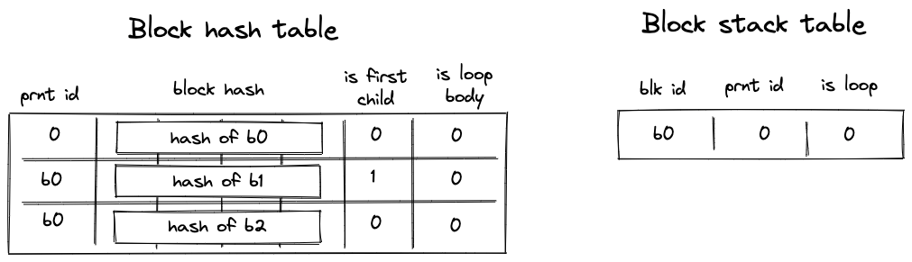
States of block hash and block stack tables after step 4:
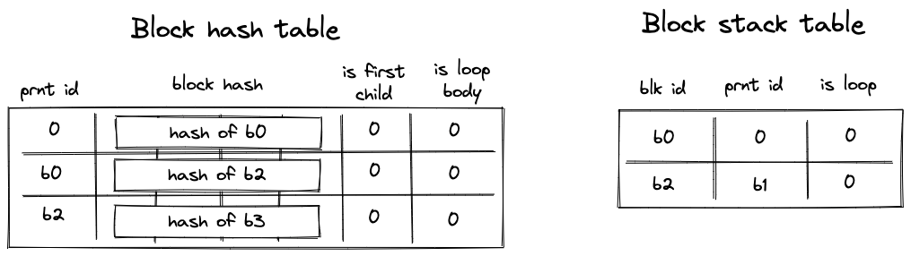
States of block hash and block stack tables after step 6:
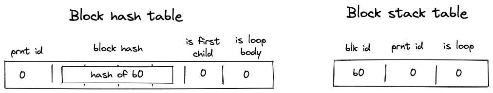
Miden VM decoder AIR constraints
In this section we describe AIR constraints for Miden VM program decoder. These constraints enforce that the execution trace generated by the prover when executing a particular program complies with the rules described in the previous section.
To refer to decoder execution trace columns, we use the names shown on the diagram below (these are the same names as in the previous section). Additionally, we denote the register containing the value at the top of the stack as .
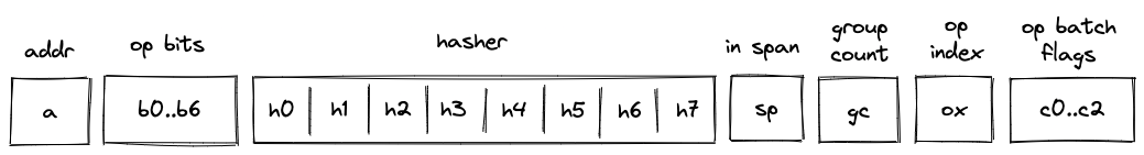
We assume that the VM exposes a flag per operation which is set to when the operation is executed, and to otherwise. The notation for such flags is . For example, when the VM executes a PUSH operation, flag . All flags are mutually exclusive - i.e., when one flag is set to all other flags are set to . The flags are computed based on values in op_bits columns.
AIR constraints for the decoder involve operations listed in the table below. For each operation we also provide the degree of the corresponding flag and the effect that the operation has on the operand stack (however, in this section we do not cover the constraints needed to enforce the correct transition of the operand stack).
| Operation | Flag | Degree | Effect on stack |
|---|---|---|---|
JOIN | 5 | Stack remains unchanged. | |
SPLIT | 5 | Top stack element is dropped. | |
LOOP | 5 | Top stack element is dropped. | |
REPEAT | 4 | Top stack element is dropped. | |
SPAN | 5 | Stack remains unchanged. | |
RESPAN | 4 | Stack remains unchanged. | |
DYN | 5 | Stack remains unchanged. | |
CALL | 4 | Stack remains unchanged. | |
SYSCALL | 4 | Stack remains unchanged. | |
END | 4 | When exiting a loop block, top stack element is dropped; otherwise, the stack remains unchanged. | |
HALT | 4 | Stack remains unchanged. | |
PUSH | 5 | An immediate value is pushed onto the stack. | |
EMIT | 5 | Stack remains unchanged. |
We also use the control flow flag exposed by the VM, which is set when any one of the above control flow operations is being executed. It has degree .
As described previously, the general idea of the decoder is that the prover provides the program to the VM by populating some of cells in the trace non-deterministically. Values in these are then used to update virtual tables (represented via multiset checks) such as block hash table, block stack table etc. Transition constraints are used to ensure that the tables are updates correctly, and we also apply boundary constraints to enforce the correct initial and final states of these tables. One of these boundary constraints binds the execution trace to the hash of the program being executed. Thus, if the virtual tables were updated correctly and boundary constraints hold, we can be convinced that the prover executed the claimed program on the VM.
In the sections below, we describe constraints according to their logical grouping. However, we start out with a set of general constraints which are applicable to multiple parts of the decoder.
General constraints
When SPLIT or LOOP operation is executed, the top of the operand stack must contain a binary value:
When a DYN operation is executed, the hasher registers must all be set to :
When REPEAT operation is executed, the value at the top of the operand stack must be :
Also, when REPEAT operation is executed, the value in column (the is_loop_body flag), must be set to . This ensures that REPEAT operation can be executed only inside a loop:
When RESPAN operation is executed, we need to make sure that the block ID is incremented by :
When END operation is executed and we are exiting a loop block (i.e., is_loop, value which is stored in , is ), the value at the top of the operand stack must be :
Also, when END operation is executed and the next operation is REPEAT, values in (the hash of the current block and the is_loop_body flag) must be copied to the next row:
A HALT instruction can be followed only by another HALT instruction:
When a HALT operation is executed, block address column must be :
Values in op_bits columns must be binary (i.e., either or ):
When the value in in_span column is set to , control flow operations cannot be executed on the VM, but when in_span flag is , only control flow operations can be executed on the VM:
Block hash computation constraints
As described previously, when the VM starts executing a new block, it also initiates computation of the block's hash. There are two separate methodologies for computing block hashes.
For join, split, and loop blocks, the hash is computed directly from the hashes of the block's children. The prover provides these child hashes non-deterministically by populating registers . For dyn, the hasher registers are populated with zeros, so the resulting hash is a constant value. The hasher is initialized using the hash chiplet, and we use the address of the hasher as the block's ID. The result of the hash is available rows down in the hasher table (i.e., at row with index equal to block ID plus ). We read the result from the hasher table at the time the END operation is executed for a given block.
For span blocks, the hash is computed by absorbing a linear sequence of instructions (organized into operation groups and batches) into the hasher and then returning the result. The prover provides operation batches non-deterministically by populating registers . Similarly to other blocks, the hasher is initialized using the hash chiplet at the start of the block, and we use the address of the hasher as the ID of the first operation batch in the block. As we absorb additional operation batches into the hasher (by executing RESPAN operation), the batch address is incremented by . This moves the "pointer" into the hasher table rows down with every new batch. We read the result from the hasher table at the time the END operation is executed for a given block.
Chiplets bus constraints
The decoder communicates with the hash chiplet via the chiplets bus. This works by dividing values of the multiset check column by the values of operations providing inputs to or reading outputs from the hash chiplet. A constraint to enforce this would look as , where is the value which defines the operation.
In constructing value of for decoder AIR constraints, we will use the following labels (see here for an explanation of how values for these labels are computed):
- this label specifies that we are starting a new hash computation.
- this label specifies that we are absorbing the next sequence of elements into an ongoing hash computation.
- this label specifies that we are reading the result of a hash computation.
To simplify constraint description, we define the following variables:
In the above, can be thought of as initiating a hasher with address and absorbing elements from the hasher state () into it. Control blocks are always padded to fill the hasher rate and as such the (first capacity register) term is set to .
It should be noted that refers to a column in the decoder, as depicted. The addresses in this column are set using the address from the hasher chiplet for the corresponding hash initialization / absorption / return. In the case of the value of the address in column in the current row of the decoder is set to equal the value of the address of the row in the hasher chiplet where the previous absorption (or initialization) occurred. is the address of the next row of the decoder, which is set to equal the address in the hasher chiplet where the absorption referred to by the label is happening.
In the above, represents the address value in the decoder which corresponds to the hasher chiplet address at which the hasher was initialized (or the last absorption took place). As such, corresponds to the hasher chiplet address at which the result is returned.
In the above, is set to when a control flow operation that signifies the initialization of a control block is being executed on the VM (only those control blocks that don't do any concurrent requests to the chiplets but). Otherwise, it is set to . An exception is made for the DYN, DYNCALL, and SYSCALL operations, since although they initialize a control block, they also run another concurrent bus request, and so are handled separately.
In the above, represents the opcode value of the opcode being executed on the virtual machine. It is calculated via a bitwise combination of the op bits. We leverage the opcode value to achieve domain separation when hashing control blocks. This is done by populating the second capacity register of the hasher with the value via the term when initializing the hasher.
Using the above variables, we define operation values as described below.
When a control block initializer operation (JOIN, SPLIT, LOOP, CALL) is executed, a new hasher is initialized and the contents of are absorbed into the hasher. As mentioned above, the opcode value is populated in the second capacity register via the term.
As mentioned previously, the value sent by the SYSCALL operation is defined separately, since in addition to communicating with the hash chiplet it must also send a kernel procedure access request to the kernel ROM chiplet. This value of this kernel procedure request is described by .
In the above, is the unique operation label of the kernel procedure call operation. The values contain the root hash of the procedure being called, which is the procedure that must be requested from the kernel ROM chiplet.
The above value sends both the hash initialization request and the kernel procedure access request to the chiplets bus when the SYSCALL operation is executed.
Similar to SYSCALL, DYN and DYNCALL are handled separately, since in addition to communicating with the hash chiplet they must also issue a memory read operation for the hash of the procedure being called.
In the above, can be thought of as , but where the values used for the hasher decoder trace registers is all 0's. represents a memory read request from memory address (the top stack element), where the result is placed in the first half of the decoder hasher trace, and where is a label that represents a memory read request.
When SPAN operation is executed, a new hasher is initialized and contents of are absorbed into the hasher. The number of operation groups to be hashed is padded to a multiple of the rate width () and so the is set to 0:
When RESPAN operation is executed, contents of (which contain the new operation batch) are absorbed into the hasher:
When END operation is executed, the hash result is copied into registers :
Using the above definitions, we can describe the constraint for computing block hashes as follows:
We need to add and subtract the sum of the relevant operation flags to ensure that when none of the flags is set to , the above constraint reduces to .
The degree of this constraint is .
Block stack table constraints
As described previously, block stack table keeps track of program blocks currently executing on the VM. Thus, whenever the VM starts executing a new block, an entry for this block is added to the block stack table. And when execution of a block completes, it is removed from the block stack table.
Adding and removing entries to/from the block stack table is accomplished as follows:
- To add an entry, we multiply the value in column by a value representing a tuple
(blk, prnt, is_loop, ctx_next, fmp_next, b0_next, b1_next, fn_hash_next). A constraint to enforce this would look as , where is the value representing the row to be added. - To remove an entry, we divide the value in column by a value representing a tuple
(blk, prnt, is_loop, ctx_next, fmp_next, b0_next, b1_next, fn_hash_next). A constraint to enforce this would look as , where is the value representing the row to be removed.
Recall that the columns
ctx_next, fmp_next, b0_next, b1_next, fn_hash_nextare only set onCALL,SYSCALL, and their correspondingENDblock. Therefore, for simplicity, we will ignore them when documenting all other block types (such that their values are set to0).
Before describing the constraints for the block stack table, we first describe how we compute the values to be added and removed from the table for each operation. In the below, for block start operations (JOIN, SPLIT, LOOP, SPAN) refers to the ID of the parent block, and refers to the ID of the starting block. For END operation, the situation is reversed: is the ID of the ending block, and is the ID of the parent block. For RESPAN operation, refers to the ID of the current operation batch, refers to the ID of the next batch, and the parent ID for both batches is set by the prover non-deterministically in register .
When JOIN operation is executed, row is added to the block stack table:
When SPLIT operation is executed, row is added to the block stack table:
When LOOP operation is executed, row is added to the block stack table if the value at the top of the operand stack is , and row is added to the block stack table if the value at the top of the operand stack is :
When SPAN operation is executed, row is added to the block stack table:
When RESPAN operation is executed, row is removed from the block stack table, and row is added to the table. The prover sets the value of register at the next row to the ID of the parent block:
When a DYN operation is executed, row is added to the block stack table:
When a DYNCALL operation is executed, row is added to the block stack table:
When a CALL or SYSCALL operation is executed, row is added to the block stack table:
When END operation is executed, how we construct the row will depend on whether the IS_CALL or IS_SYSCALL values are set (stored in registers and respectively). If they are not set, then row is removed from the block span table (where contains the is_loop flag); otherwise, row .
Using the above definitions, we can describe the constraint for updating the block stack table as follows:
We need to add and subtract the sum of the relevant operation flags from each side to ensure that when none of the flags is set to , the above constraint reduces to .
The degree of this constraint is .
In addition to the above transition constraint, we also need to impose boundary constraints against the column to make sure the first and the last values in the column are set to . This enforces that the block stack table starts and ends in an empty state.
Block hash table constraints
As described previously, when the VM starts executing a new program block, it adds hashes of the block's children to the block hash table. And when the VM finishes executing a block, it removes the block's hash from the block hash table. This means that the block hash table gets updated when we execute the JOIN, SPLIT, LOOP, REPEAT, DYN, and END operations (executing SPAN operation does not affect the block hash table because a span block has no children).
Adding and removing entries to/from the block hash table is accomplished as follows:
- To add an entry, we multiply the value in column by a value representing a tuple
(prnt_id, block_hash, is_first_child, is_loop_body). A constraint to enforce this would look as , where is the value representing the row to be added. - To remove an entry, we divide the value in column by a value representing a tuple
(prnt_id, block_hash, is_first_child, is_loop_body). A constraint to enforce this would look as , where is the value representing the row to be removed.
To simplify constraint descriptions, we define values representing left and right children of a block as follows:
Graphically, this looks like so:
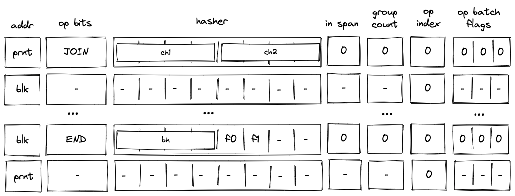
In a similar manner, we define a value representing the result of hash computation as follows:
1
Above, refers to the value in the IS_LOOP_BODY column (already constrained to be 0 or 1), located in . Also, note that we are not adding a flag indicating whether the block is the first child of a join block (i.e., term is missing). It will be added later on.
Using the above variables, we define row values to be added to and removed from the block hash table as follows.
When JOIN operation is executed, hashes of both child nodes are added to the block hash table. We add term to the first child value to differentiate it from the second child (i.e., this sets is_first_child to ):
When SPLIT operation is executed and the top of the stack is , hash of the true branch is added to the block hash table, but when the top of the stack is , hash of the false branch is added to the block hash table:
When LOOP operation is executed and the top of the stack is , hash of loop body is added to the block hash table. We add term to indicate that the child is a body of a loop. The below also means that if the top of the stack is , nothing is added to the block hash table as the expression evaluates to :
When REPEAT operation is executed, hash of loop body is added to the block hash table. We add term to indicate that the child is a body of a loop:
When DYN, DYNCALL, CALL or SYSCALL operation is executed, the hash of the child is added to the block hash table. In all cases, this child is found in the first half of the decoder hasher state.
When END operation is executed, hash of the completed block is removed from the block hash table. However, we also need to differentiate between removing the first and the second child of a join block. We do this by looking at the next operation. Specifically, if the next operation is neither END nor REPEAT nor HALT, we know that another block is about to be executed, and thus, we have just finished executing the first child of a join block. Thus, if the next operation is neither END nor REPEAT nor HALT we need to set the term for coefficient to as shown below:
Using the above definitions, we can describe the constraint for updating the block hash table as follows:
We need to add and subtract the sum of the relevant operation flags from each side to ensure that when none of the flags is set to , the above constraint reduces to .
The degree of this constraint is .
In addition to the above transition constraint, we also need to set the following boundary constraints against the column:
- The first value in the column represents a row for the entire program. Specifically, the row tuple would be
(0, program_hash, 0, 0). This row should be removed from the table when the lastENDoperation is executed. - The last value in the column is - i.e., the block hash table is empty.
Span block
Span block constraints ensure proper decoding of span blocks. In addition to the block stack table constraints and block hash table constraints described previously, decoding of span blocks requires constraints described below.
In-span column constraints
The in_span column (denoted as ) is used to identify rows which execute non-control flow operations. The values in this column are set as follows:
- Executing a
SPANoperation sets the value ofin_spancolumn to . - The value remains until the
ENDoperation is executed. - If
RESPANoperation is executed betweenSPANandENDoperations, in the row at whichRESPANoperation is executedin_spanis set to . It is then reset to in the following row. - In all other cases, value in the
in_spancolumn should be .
The picture below illustrates the above rules.
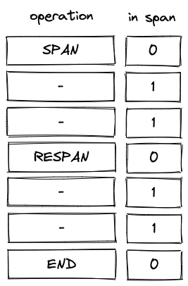
To enforce the above rules we need the following constraints.
When executing SPAN or RESPAN operation, the next value in column must be set to :
When the next operation is END or RESPAN, the next value in column must be set .
In all other cases, the value in column must be copied over to the next row:
Additionally, we will need to impose a boundary constraint which specifies that the first value in . Note, however, that we do not need to impose a constraint ensuring that values in are binary - this will follow naturally from the above constraints.
Also, note that the combination of the above constraints makes it impossible to execute END or RESPAN operations right after SPAN or RESPAN operations.
Block address constraints
When we are inside a span block, values in block address columns (denoted as ) must remain the same. This can be enforced with the following constraint:
Notice that this constraint does not apply when we execute any of the control flow operations. For such operations, the prover sets the value of the column non-deterministically, except for the RESPAN operation. For the RESPAN operation the value in the column is incremented by , which is enforced by a constraint described previously.
Notice also that this constraint implies that when the next operation is the END operation, the value in the column must also be copied over to the next row. This is exactly the behavior we want to enforce so that when the END operation is executed, the block address is set to the address of the current span batch.
Group count constraints
The group_count column (denoted as ) is used to keep track of the number of operation groups which remains to be executed in a span block.
In the beginning of a span block (i.e., when SPAN operation is executed), the prover sets the value of non-deterministically. This value is subsequently decremented according to the rules described below. By the time we exit the span block (i.e., when END operation is executed), the value in must be .
The rules for decrementing values in the column are as follows:
- The count cannot be decremented by more than in a single row.
- When an operation group is fully executed (which happens when inside a span block), the count is decremented by .
- When
SPAN,RESPAN,EMITorPUSHoperations are executed, the count is decremented by .
Note that these rules imply that the EMIT and PUSH operations cannot be the last operation in an operation group (otherwise the count would have to be decremented by ).
To simplify the description of the constraints, we will define the following variable:
Using this variable, we can describe the constraints against the column as follows:
Inside a span block, group count can either stay the same or decrease by one:
When group count is decremented inside a span block, either must be (we consumed all operations in a group) or we must be executing an operation with an immediate value:
Notice that the above constraint does not preclude and from being true at the same time. If this happens, op group decoding constraints (described here) will force that the operation following the operation with an immediate value is a NOOP.
When executing a SPAN, a RESPAN, or an operation with an immediate value, group count must be decremented by :
If the next operation is either an END or a RESPAN, group count must remain the same:
When an END operation is executed, group count must be :
Op group decoding constraints
Inside a span block, register is used to keep track of operations to be executed in the current operation group. The value of this register is set by the prover non-deterministically at the time when the prover executes a SPAN or a RESPAN operation, or when processing of a new operation group within a batch starts. The picture below illustrates this.
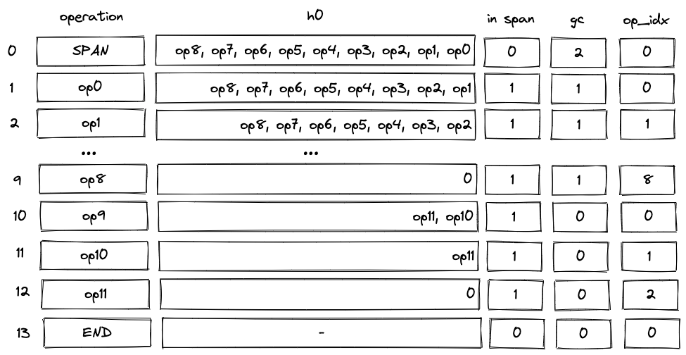
In the above:
- The prover sets the value of non-deterministically at row . The value is set to an operation group containing operations
op0throughop8. - As we start executing the group, at every row we "remove" the least significant operation from the group. This can be done by subtracting opcode of the operation from the group, and then dividing the result by .
- By row the group is fully executed. This decrements the group count and set
op_indexto (constraints againstop_indexcolumn are described in the next section). - At row we start executing the next group with operations
op9throughop11. In this case, the prover populates with the group having its first operation (op9) already removed, and sets theop_bitsregisters to the value encodingop9. - By row this group is also fully executed.
To simplify the description of the constraints, we define the following variables:
is just an opcode value implied by the values in op_bits registers. is a flag which is set to when the group count within a span block does not change. We multiply it by to make sure the flag is when we are about to end decoding of an operation batch. Note that flag is mutually exclusive with , , and flags as these three operations decrement the group count.
Using these variables, we can describe operation group decoding constraints as follows:
When a SPAN, a RESPAN, or an operation with an immediate value is executed or when the group count does not change, the value in should be decremented by the value of the opcode in the next row.
Notice that when the group count does change, and we are not executing , , or operations, no constraints are placed against , and thus, the prover can populate this register non-deterministically.
When we are in a span block and the next operation is END or RESPAN, the current value in column must be .
Op index constraints
The op_index column (denoted as ) tracks index of an operation within its operation group. It is used to ensure that the number of operations executed per group never exceeds . The index is zero-based, and thus, the possible set of values for is between and (both inclusive).
To simplify the description of the constraints, we will define the following variables:
The value of is set to when we are about to start executing a new operation group (i.e., group count is decremented but we did not execute an operation with an immediate value). Using these variables, we can describe the constraints against the column as follows.
When executing SPAN or RESPAN operations the next value of op_index must be set to :
When starting a new operation group inside a span block, the next value of op_index must be set to . Note that we multiply by to exclude the cases when the group count is decremented because of SPAN or RESPAN operations:
When inside a span block but not starting a new operation group, op_index must be incremented by . Note that we multiply by to exclude the cases when we are about to exit processing of an operation batch (i.e., the next operation is either END or RESPAN):
Values of op_index must be in the range .
Op batch flags constraints
Operation batch flag columns (denoted , , and ) are used to specify how many operation groups are present in an operation batch. This is relevant for the last batch in a span block (or the first batch if there is only one batch in a block) as all other batches should be completely full (i.e., contain 8 operation groups).
These columns are used to define the following 4 flags:
- : there are 8 operation groups in the batch.
- : there are 4 operation groups in the batch.
- : there are 2 operation groups in the batch.
- : there is only 1 operation groups in the batch.
Notice that the degree of is , while the degree of the remaining flags is .
These flags can be set to only when we are executing SPAN or RESPAN operations as this is when the VM starts processing new operation batches. Also, for a given flag we need to ensure that only the specified number of operations groups are present in a batch. This can be done with the following constraints.
All batch flags must be binary:
When SPAN or RESPAN operations is executed, one of the batch flags must be set to .
When neither SPAN nor RESPAN is executed, all batch flags must be set to .
When we have at most 4 groups in a batch, registers should be set to 's.
When we have at most 2 groups in a batch, registers and should also be set to 's.
When we have at most 1 groups in a batch, register should also be set to .
Op group table constraints
Op group table is used to ensure that all operation groups in a given batch are consumed before a new batch is started (i.e., via a RESPAN operation) or the execution of a span block is complete (i.e., via an END operation). The op group table is updated according to the following rules:
- When a new operation batch is started, we add groups from this batch to the table. To add a group to the table, we multiply the value in column by a value representing a tuple
(batch_id, group_pos, group). A constraint to enforce this would look as , where is the value representing the row to be added. Depending on the batch, we may need to add multiple groups to the table (i.e., ). Flags , , , and are used to define how many groups to add. - When a new operation group starts executing or when an immediate value is consumed, we remove the corresponding group from the table. To do this, we divide the value in column by a value representing a tuple
(batch_id, group_pos, group). A constraint to enforce this would look as , where is the value representing the row to be removed.
To simplify constraint descriptions, we first define variables representing the rows to be added to and removed from the op group table.
When a SPAN or a RESPAN operation is executed, we compute the values of the rows to be added to the op group table as follows:
Where . Thus, defines row value for group in , defines row value for group etc. Note that batch address column comes from the next row of the block address column ().
We compute the value of the row to be removed from the op group table as follows:
In the above, the value of the group is computed as . This basically says that when we execute a PUSH or EMIT operation we need to remove the immediate value from the table. For PUSH, this value is at the top of the stack (column ) in the next row; for EMIT, it is found in . However, when we are executing neither a PUSH nor EMIT operation, the value to be removed is an op group value which is a combination of values in and op_bits columns (also in the next row). Note also that value for batch address comes from the current value in the block address column (), and the group position comes from the current value of the group count column ().
We also define a flag which is set to when a group needs to be removed from the op group table.
The above says that we remove groups from the op group table whenever group count is decremented. We multiply by to exclude the cases when the group count is decremented due to SPAN or RESPAN operations.
Using the above variables together with flags , , defined in the previous section, we describe the constraint for updating op group table as follows (note that we do not use flag as when a batch consists of a single group, nothing is added to the op group table):
The above constraint specifies that:
- When
SPANorRESPANoperations are executed, we add between and groups to the op group table; else, leave untouched. - When group count is decremented inside a span block, we remove a group from the op group table; else, leave untouched.
The degree of this constraint is .
In addition to the above transition constraint, we also need to impose boundary constraints against the column to make sure the first and the last value in the column is set to . This enforces that the op group table table starts and ends in an empty state.
Operand stack
Miden VM is a stack machine. The stack is a push-down stack of practically unlimited depth (in practical terms, the depth will never exceed ), but only the top items are directly accessible to the VM. Items on the stack are elements in a prime field with modulus .
To keep the constraint system for the stack manageable, we impose the following rules:
- All operations executed on the VM can shift the stack by at most one item. That is, the end result of an operation must be that the stack shrinks by one item, grows by one item, or the number of items on the stack stays the same.
- Stack depth must always be greater than or equal to . At the start of program execution, the stack is initialized with exactly input values, all of which could be 's.
- By the end of program execution, exactly items must remain on the stack (again, all of them could be 's). These items comprise the output of the program.
To ensure that managing stack depth does not impose significant burden, we adopt the following rule:
- When the stack depth is , removing additional items from the stack does not change its depth. To keep the depth at , 's are inserted into the deep end of the stack for each removed item.
Stack representation
The VM allocates trace columns for the stack. The layout of the columns is illustrated below.
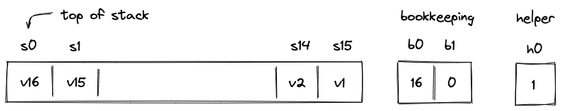
The meaning of the above columns is as follows:
- are the columns representing the top slots of the stack.
- Column contains the number of items on the stack (i.e., the stack depth). In the above picture, there are 16 items on the stacks, so .
- Column contains an address of a row in the "overflow table" in which we'll store the data that doesn't fit into the top slots. When , it means that all stack data fits into the top slots of the stack.
- Helper column is used to ensure that stack depth does not drop below . Values in this column are set by the prover non-deterministically to when , and to any other value otherwise.
Overflow table
To keep track of the data which doesn't fit into the top stack slots, we'll use an overflow table. This will be a virtual table. To represent this table, we'll use a single auxiliary column .
The table itself can be thought of as having 3 columns as illustrated below.
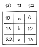
The meaning of the columns is as follows:
- Column contains row address. Every address in the table must be unique.
- Column contains the value that overflowed the stack.
- Column contains the address of the row containing the value that overflowed the stack right before the value in the current row. For example, in the picture above, first value overflowed the stack, then overflowed the stack, and then value overflowed the stack. Thus, row with value points back to the row with value , and row with value points back to the row with value .
To reduce a table row to a single value, we'll compute a randomized product of column values as follows:
Then, when row is added to the table, we'll update the value in the column like so:
Analogously, when row is removed from the table, we'll update the value in column like so:
The initial value of is set to . Thus, if by the time Miden VM finishes executing a program the table is empty (we added and then removed exactly the same set of rows), will also be equal to .
There are a couple of other rules we'll need to enforce:
- We can delete a row only after the row has been inserted into the table.
- We can't insert a row with the same address twice into the table (even if the row was inserted and then deleted).
How these are enforced will be described a bit later.
Right shift
If an operation adds data to the stack, we say that the operation caused a right shift. For example, PUSH and DUP operations cause a right shift. Graphically, this looks like so:
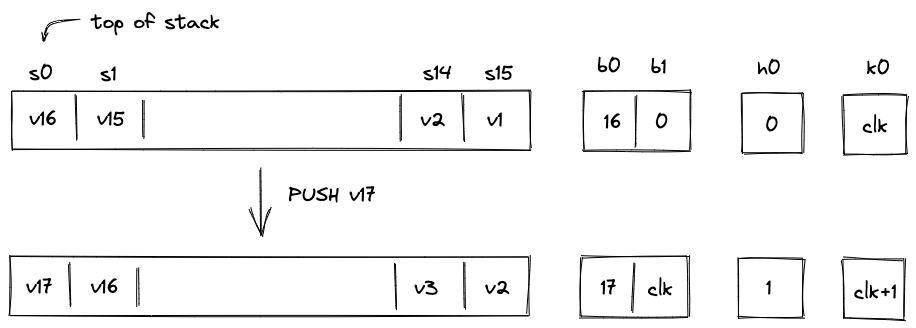
Here, we pushed value onto the stack. All other values on the stack are shifted by one slot to the right and the stack depth increases by . There is not enough space at the top of the stack for all values, thus, needs to be moved to the overflow table.
To do this, we need to rely on another column: . This is a system column which keeps track of the current VM cycle. The value in this column is simply incremented by with every step.
The row we want to add to the overflow table is defined by tuple , and after it is added, the table would look like so:
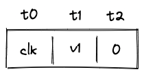
The reason we use VM clock cycle as row address is that the clock cycle is guaranteed to be unique, and thus, the same row can not be added to the table twice.
Let's push another item onto the stack:
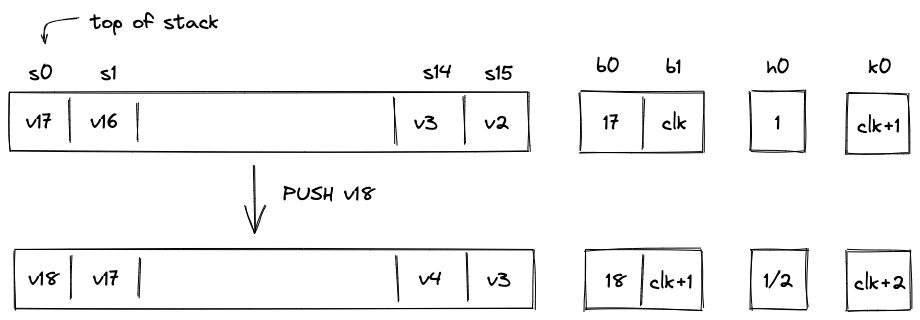
Again, as we push onto the stack, all items on the stack are shifted to the right, and now needs to be moved to the overflow table. The tuple we want to insert into the table now is . After the operation, the overflow table will look like so:
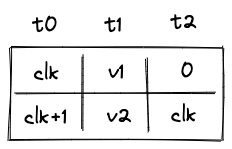
Notice that for row which contains value points back to the row with address .
Overall, during a right shift we do the following:
- Increment stack depth by .
- Shift stack columns right by slot.
- Add a row to the overflow table described by tuple .
- Set the next value of to the current value of .
Also, as mentioned previously, the prover sets values in non-deterministically to .
Left shift
If an operation removes an item from the stack, we say that the operation caused a left shift. For example, a DROP operation causes a left shift. Assuming the stack is in the state we left it at the end of the previous section, graphically, this looks like so:
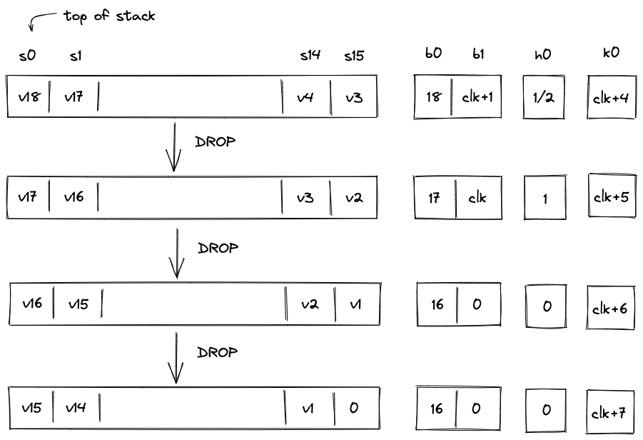
Overall, during the left shift we do the following:
- When stack depth is greater than :
- Decrement stack depth by .
- Shift stack columns left by slot.
- Remove a row from the overflow table with equal to the current value of .
- Set the next value of to the value in of the removed overflow table row.
- Set the next value of to the value in of the removed overflow table row.
- When the stack depth is equal to :
- Keep the stack depth the same.
- Shift stack columns left by slot.
- Set the value of to .
- Set the value to to (or any other value).
If the stack depth becomes (or remains) , the prover can set to any value (e.g., ). But if the depth is greater than the prover sets to .
AIR Constraints
To simplify constraint descriptions, we'll assume that the VM exposes two binary flag values described below.
| Flag | Degree | Description |
|---|---|---|
| 6 | When this flag is set to , the instruction executing on the VM is performing a "right shift". | |
| 5 | When this flag is set to , the instruction executing on the VM is performing a "left shift". |
These flags are mutually exclusive. That is, if , then and vice versa. However, both flags can be set to simultaneously. This happens when the executed instruction does not shift the stack. How these flags are computed is described here.
Stack overflow flag
Additionally, we'll define a flag to indicate whether the overflow table contains values. This flag will be set to when the overflow table is empty, and to otherwise (i.e., when stack depth ). This flag can be computed as follows:
To ensure that this flag is set correctly, we need to impose the following constraint:
The above constraint can be satisfied only when either of the following holds:
- , in which case evaluates to , regardless of the value of .
- , in which case cannot be equal to (and must be set to ).
Stack depth constraints
To make sure stack depth column is updated correctly, we need to impose the following constraints:
| Condition | Constraint__ | Description |
|---|---|---|
| When the stack is shifted to the right, stack depth should be incremented by . | ||
| | When the stack is shifted to the left and the overflow table is not empty, stack depth should be decremented by . | |
| otherwise | In all other cases, stack depth should not change. |
We can combine the above constraints into a single expression as follows:
Overflow table constraints
When the stack is shifted to the right, a tuple should be added to the overflow table. We will denote value of the row to be added to the table as follows:
When the stack is shifted to the left, a tuple should be removed from the overflow table. We will denote value of the row to be removed from the table as follows.
Using the above variables, we can ensure that right and left shifts update the overflow table correctly by enforcing the following constraint:
The above constraint reduces to the following under various flag conditions:
| Condition | Applied constraint |
|---|---|
| , , | |
| , , | |
| , , | |
| , , |
Notice that in the case of the left shift, the constraint forces the prover to set the next values of and to values and of the row removed from the overflow table.
In case of a right shift, we also need to make sure that the next value of is set to the current value of . This can be done with the following constraint:
In case of a left shift, when the overflow table is empty, we need to make sure that a is "shifted in" from the right (i.e., is set to ). This can be done with the following constraint:
Boundary constraints
In addition to the constraints described above, we also need to enforce the following boundary constraints:
- at the first and at the last row of execution trace.
- at the first and at the last row of execution trace.
- at the first and at the last row of execution trace.
Stack operation constraints
In addition to the constraints described in the previous section, we need to impose constraints to check that each VM operation is executed correctly.
For this purpose the VM exposes a set of operation-specific flags. These flags are set to when a given operation is executed, and to otherwise. The naming convention for these flags is . For example, would be set to when DUP operation is executed, and to otherwise. Operation flags are discussed in detail in the section below.
To describe how operation-specific constraints work, let's use an example with DUP operation. This operation pushes a copy of the top stack item onto the stack. The constraints we need to impose for this operation are as follows:
The first constraint enforces that the top stack item in the next row is the same as the top stack item in the current row. The second constraint enforces that all stack items (starting from item ) are shifted to the right by . We also need to impose all the constraints discussed in the previous section, be we omit them here.
Let's write similar constraints for DUP1 operation, which pushes a copy of the second stack item onto the stack:
It is easy to notice that while the first constraint changed, the second constraint remained the same - i.e., we are still just shifting the stack to the right.
In fact, for most operations it makes sense to make a distinction between constraints unique to the operation vs. more general constraints which enforce correct behavior for the stack items not affected by the operation. In the subsequent sections we describe in detail only the former constraints, and provide high-level descriptions of the more general constraints. Specifically, we indicate how the operation affects the rest of the stack (e.g., shifts right starting from position ).
Operation flags
As mentioned above, operation flags are used as selectors to enforce operation-specific constraints. That is, they turn on relevant constraints for a given operation. In total, the VM provides unique operations, and thus, there are operation flags (not all of them currently used).
Operation flags are mutually exclusive. That is, if one flag is set to , all other flags are set to . Also, one of the flags is always guaranteed to be set to .
To compute values of operation flags we use op bits registers located in the decoder. These registers contain binary representations of operation codes (opcodes). Each opcode consists of bits, and thus, there are op bits registers. We denote these registers as . The values are computed by multiplying the op bit registers in various combinations. Notice that binary encoding down below is showed in big-endian order, so the flag bits correspond to the reverse order of the op bits registers, from to .
For example, the value of the flag for NOOP, which is encoded as 0000000, is computed as follows:
While the value of the DROP operation, which is encoded as 0101001 is computed as follows:
As can be seen from above, the degree for both of these flags is . Since degree of constraints in Miden VM can go up to , this means that operation-specific constraints cannot exceed degree . However, there are some operations which require constraints of higher degree (e.g., or even ). To support such constraints, we adopt the following scheme.
We organize the operations into groups as shown below and also introduce two extra registers and for degree reduction:
| # of ops | degree | |||||||||
|---|---|---|---|---|---|---|---|---|---|---|
| 0 | x | x | x | x | x | x | 0 | 0 | 64 | 7 |
| 1 | 0 | 0 | x | x | x | - | 0 | 0 | 8 | 6 |
| 1 | 0 | 1 | x | x | x | x | 1 | 0 | 16 | 5 |
| 1 | 1 | x | x | x | - | - | 0 | 1 | 8 | 4 |
In the above:
- Operation flags for operations in the first group (with prefix
0), are computed using all op bits, and thus their degree is . - Operation flags for operations in the second group (with prefix
100), are computed using only the first op bits, and thus their degree is . - Operation flags for operations in the third group (with prefix
101), are computed using all op bits. We use the extra register (which is set to ) to reduce the degree by . Thus, the degree of op flags in this group is . - Operation flags for operations in the fourth group (with prefix
11), are computed using only the first op bits. We use the extra register (which is set to ) to reduce the degree by . Thus, the degree of op flags in this group is .
How operations are distributed between these groups is described in the sections below.
No stack shift operations
This group contains operations which do not shift the stack (this is almost all such operations). Since the op flag degree for these operations is , constraints for these operations cannot exceed degree .
| Operation | Opcode value | Binary encoding | Operation group | Flag degree |
|---|---|---|---|---|
NOOP | 000_0000 | System ops | ||
EQZ | 000_0001 | Field ops | ||
NEG | 000_0010 | Field ops | ||
INV | 000_0011 | Field ops | ||
INCR | 000_0100 | Field ops | ||
NOT | 000_0101 | Field ops | ||
FMPADD | 000_0110 | System ops | ||
MLOAD | 000_0111 | I/O ops | ||
SWAP | 000_1000 | Stack ops | ||
CALLER | 000_1001 | System ops | ||
MOVUP2 | 000_1010 | Stack ops | ||
MOVDN2 | 000_1011 | Stack ops | ||
MOVUP3 | 000_1100 | Stack ops | ||
MOVDN3 | 000_1101 | Stack ops | ||
ADVPOPW | 000_1110 | I/O ops | ||
EXPACC | 000_1111 | Field ops | ||
MOVUP4 | 001_0000 | Stack ops | ||
MOVDN4 | 001_0001 | Stack ops | ||
MOVUP5 | 001_0010 | Stack ops | ||
MOVDN5 | 001_0011 | Stack ops | ||
MOVUP6 | 001_0100 | Stack ops | ||
MOVDN6 | 001_0101 | Stack ops | ||
MOVUP7 | 001_0110 | Stack ops | ||
MOVDN7 | 001_0111 | Stack ops | ||
SWAPW | 001_1000 | Stack ops | ||
EXT2MUL | 001_1001 | Field ops | ||
MOVUP8 | 001_1010 | Stack ops | ||
MOVDN8 | 001_1011 | Stack ops | ||
SWAPW2 | 001_1100 | Stack ops | ||
SWAPW3 | 001_1101 | Stack ops | ||
SWAPDW | 001_1110 | Stack ops | ||
<unused> | 001_1111 |
Left stack shift operations
This group contains operations which shift the stack to the left (i.e., remove an item from the stack). Most of left-shift operations are contained in this group. Since the op flag degree for these operations is , constraints for these operations cannot exceed degree .
| Operation | Opcode value | Binary encoding | Operation group | Flag degree |
|---|---|---|---|---|
ASSERT | 010_0000 | System ops | ||
EQ | 010_0001 | Field ops | ||
ADD | 010_0010 | Field ops | ||
MUL | 010_0011 | Field ops | ||
AND | 010_0100 | Field ops | ||
OR | 010_0101 | Field ops | ||
U32AND | 010_0110 | u32 ops | ||
U32XOR | 010_0111 | u32 ops | ||
FRIE2F4 | 010_1000 | Crypto ops | ||
DROP | 010_1001 | Stack ops | ||
CSWAP | 010_1010 | Stack ops | ||
CSWAPW | 010_1011 | Stack ops | ||
MLOADW | 010_1100 | I/O ops | ||
MSTORE | 010_1101 | I/O ops | ||
MSTOREW | 010_1110 | I/O ops | ||
FMPUPDATE | 010_1111 | System ops |
Right stack shift operations
This group contains operations which shift the stack to the right (i.e., push a new item onto the stack). Most of right-shift operations are contained in this group. Since the op flag degree for these operations is , constraints for these operations cannot exceed degree .
| Operation | Opcode value | Binary encoding | Operation group | Flag degree |
|---|---|---|---|---|
PAD | 011_0000 | Stack ops | ||
DUP | 011_0001 | Stack ops | ||
DUP1 | 011_0010 | Stack ops | ||
DUP2 | 011_0011 | Stack ops | ||
DUP3 | 011_0100 | Stack ops | ||
DUP4 | 011_0101 | Stack ops | ||
DUP5 | 011_0110 | Stack ops | ||
DUP6 | 011_0111 | Stack ops | ||
DUP7 | 011_1000 | Stack ops | ||
DUP9 | 011_1001 | Stack ops | ||
DUP11 | 011_1010 | Stack ops | ||
DUP13 | 011_1011 | Stack ops | ||
DUP15 | 011_1100 | Stack ops | ||
ADVPOP | 011_1101 | I/O ops | ||
SDEPTH | 011_1110 | I/O ops | ||
CLK | 011_1111 | System ops |
u32 operations
This group contains u32 operations. These operations are grouped together because all of them require range checks. The constraints for range checks are of degree , however, since all these operations require them, we can define a flag with common prefix 100 to serve as a selector for the range check constraints. The value of this flag is computed as follows:
The degree of this flag is , which is acceptable for a selector for degree constraints.
| Operation | Opcode value | Binary encoding | Operation group | Flag degree |
|---|---|---|---|---|
U32ADD | 100_0000 | u32 ops | ||
U32SUB | 100_0010 | u32 ops | ||
U32MUL | 100_0100 | u32 ops | ||
U32DIV | 100_0110 | u32 ops | ||
U32SPLIT | 100_1000 | u32 ops | ||
U32ASSERT2 | 100_1010 | u32 ops | ||
U32ADD3 | 100_1100 | u32 ops | ||
U32MADD | 100_1110 | u32 ops |
As mentioned previously, the last bit of the opcode is not used in computation of the flag for these operations. We force this bit to always be set to with the following constraint:
Putting these operations into a group with flag degree is important for two other reasons:
- Constraints for the
U32SPLIToperation have degree . Thus, the degree of the op flag for this operation cannot exceed . - Operations
U32ADD3andU32MADDshift the stack to the left. Thus, having these two operations in this group and putting them under the common prefix10011allows us to create a common flag for these operations of degree (recall that the left-shift flag cannot exceed degree ).
High-degree operations
This group contains operations which require constraints with degree up to . All operation bits are used for these flags. The extra column is used for degree reduction of the three high-degree bits.
| Operation | Opcode value | Binary encoding | Operation group | Flag degree |
|---|---|---|---|---|
HPERM | 101_0000 | Crypto ops | ||
MPVERIFY | 101_0001 | Crypto ops | ||
PIPE | 101_0010 | I/O ops | ||
MSTREAM | 101_0011 | I/O ops | ||
SPLIT | 101_0100 | Flow control ops | ||
LOOP | 101_0101 | Flow control ops | ||
SPAN | 101_0110 | Flow control ops | ||
JOIN | 101_0111 | Flow control ops | ||
DYN | 101_1000 | Flow control ops | ||
HORNEREXT | 101_1001 | Crypto ops | ||
EMIT | 101_1010 | System ops | ||
PUSH | 101_1011 | I/O ops | ||
DYNCALL | 101_1100 | Flow control ops | ||
<unused> | 101_1101 | |||
<unused> | 101_1110 | |||
<unused> | 101_1111 |
Note that the SPLIT and LOOP operations are grouped together under the common prefix 101010, and thus can have a common flag of degree (using for degree reduction). This is important because both of these operations shift the stack to the left.
Also, we need to make sure that extra register , which is used to reduce the flag degree by , is set to when , , and :
Very high-degree operations
This group contains operations which require constraints with degree up to .
| Operation | Opcode value | Binary encoding | Operation group | Flag degree |
|---|---|---|---|---|
MRUPDATE | 110_0000 | Crypto ops | ||
HORNERBASE | 110_0100 | Crypto ops | ||
SYSCALL | 110_1000 | Flow control ops | ||
CALL | 110_1100 | Flow control ops | ||
END | 111_0000 | Flow control ops | ||
REPEAT | 111_0100 | Flow control ops | ||
RESPAN | 111_1000 | Flow control ops | ||
HALT | 111_1100 | Flow control ops |
As mentioned previously, the last two bits of the opcode are not used in computation of the flag for these operations. We force these bits to always be set to with the following constraints:
Also, we need to make sure that extra register , which is used to reduce the flag degree by , is set to when both and columns are set to :
Composite flags
Using the operation flags defined above, we can compute several composite flags which are used by various constraints in the VM.
Shift right flag
The right-shift flag indicates that an operation shifts the stack to the right. This flag is computed as follows:
In the above, evaluates to for all right stack shift operations described previously. This works because all these operations have a common prefix 011. We also need to add in flags for other operations which shift the stack to the right but are not a part of the above group (e.g., PUSH operation).
Shift left flag
The left-shift flag indicates that a given operation shifts the stack to the left. To simplify the description of this flag, we will first compute the following intermediate variables:
A flag which is set to when or :
A flag which is set to when or :
Using the above variables, we compute left-shift flag as follows:
In the above:
- evaluates to for all left stack shift operations described previously. This works because all these operations have a common prefix
010. - is the helper register in the decoder which is set to when we are exiting a
LOOPblock, and to otherwise.
Thus, similarly to the right-shift flag, we compute the value of the left-shift flag based on the prefix of the operation group which contains most left shift operations, and add in flag values for other operations which shift the stack to the left but are not a part of this group.
Control flow flag
The control flow flag is set to when a control flow operation is being executed by the VM, and to otherwise. Naively, this flag can be computed as follows:
However, this can be computed more efficiently via the common operation prefixes for the two groups of control flow operations as follows.
Immediate value flag
The immediate value flag is set to 1 when an operation has an immediate value, and 0 otherwise:
Note that the ASSERT, MPVERIFY and other operations have immediate values too. However, these immediate values are not included in the MAST digest, and hence are not considered for the flag.
System Operations
In this section we describe the AIR constraints for Miden VM system operations.
NOOP
The NOOP operation advances the cycle counter but does not change the state of the operand stack (i.e., the depth of the stack and the values on the stack remain the same).
The NOOP operation does not impose any constraints besides the ones needed to ensure that the entire state of the stack is copied over. This constraint looks like so:
EMIT
Similarly to NOOP, the EMIT operation advances the cycle counter but does not change the state of the operand stack (i.e., the depth of the stack and the values on the stack remain the same).
The EMIT operation does not impose any constraints besides the ones needed to ensure that the entire state of the stack is copied over. This constraint looks like so:
Additionally, the prover puts EMIT's immediate value in the first user op helper register non-deterministically. The Op Group Table is responsible for ensuring that the prover sets the appropriate value.
ASSERT
The ASSERT operation pops an element off the stack and checks if the popped element is equal to . If the element is not equal to , program execution fails.
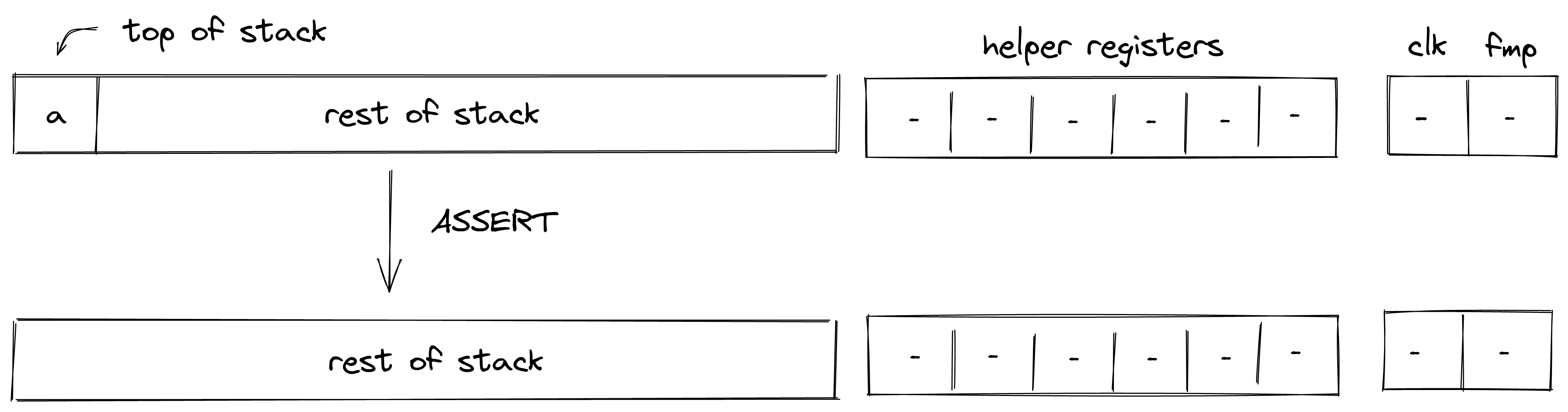
Stack transition for this operation must satisfy the following constraints:
The effect on the rest of the stack is:
- Left shift starting from position .
FMPADD
The FMPADD operation pops an element off the stack, adds the current value of the fmp register to it, and pushes the result back onto the stack. The diagram below illustrates this graphically.
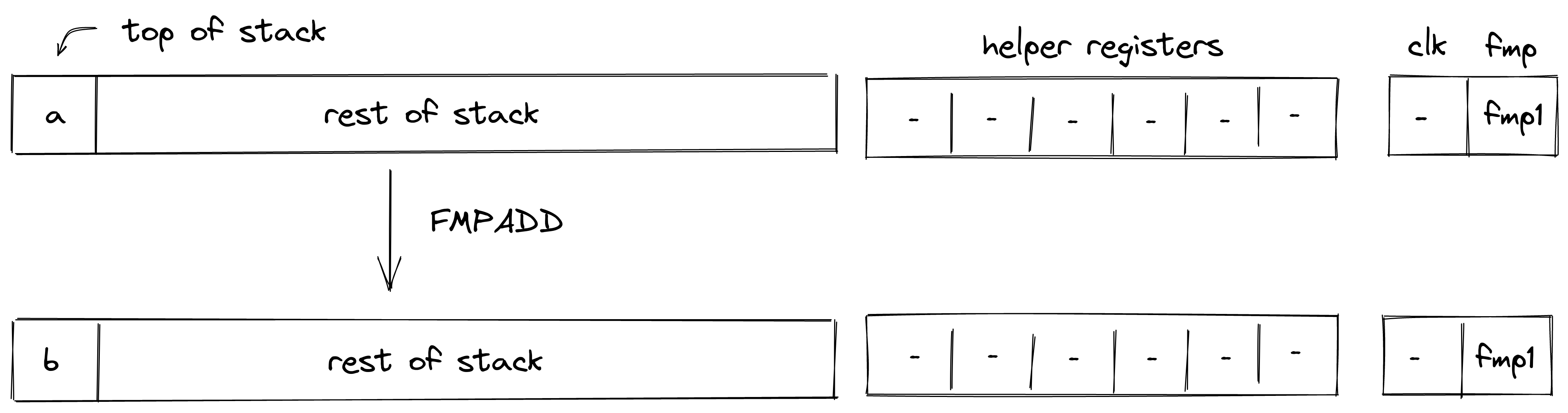
Stack transition for this operation must satisfy the following constraints:
The effect on the rest of the stack is:
- No change starting from position .
FMPUPDATE
The FMPUPDATE operation pops an element off the stack and adds it to the current value of the fmp register. The diagram below illustrates this graphically.
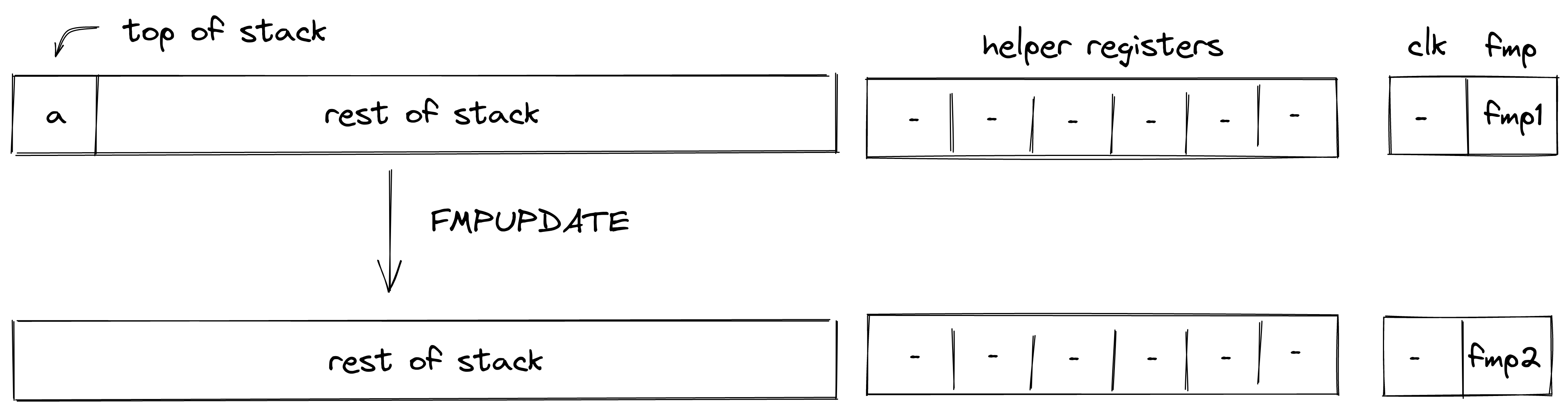
The stack transition for this operation must follow the following constraint:
The effect on the rest of the stack is:
- Left shift starting from position .
CLK
The CLK operation pushes the current value of the clock cycle onto the stack. The diagram below illustrates this graphically.
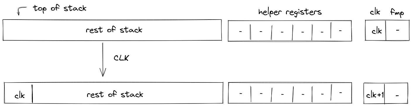
The stack transition for this operation must follow the following constraint:
The effect on the rest of the stack is:
- Right shift starting from position .
Field Operations
In this section we describe the AIR constraints for Miden VM field operations (i.e., arithmetic operations over field elements).
ADD
Assume and are the elements at the top of the stack. The ADD operation computes . The diagram below illustrates this graphically.
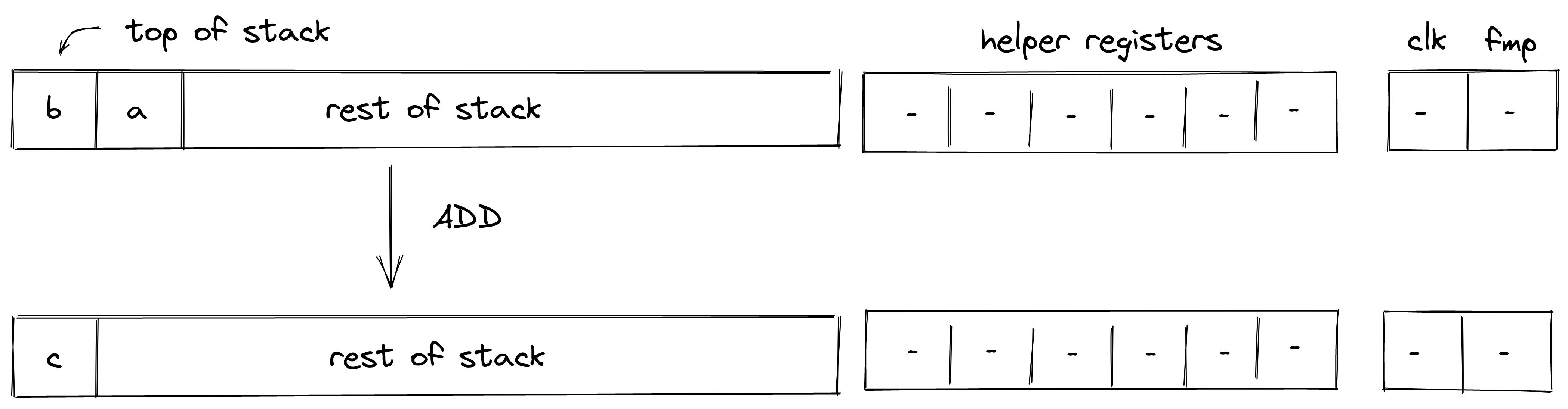
Stack transition for this operation must satisfy the following constraints:
The effect on the rest of the stack is:
- Left shift starting from position .
NEG
Assume is the element at the top of the stack. The NEG operation computes . The diagram below illustrates this graphically.
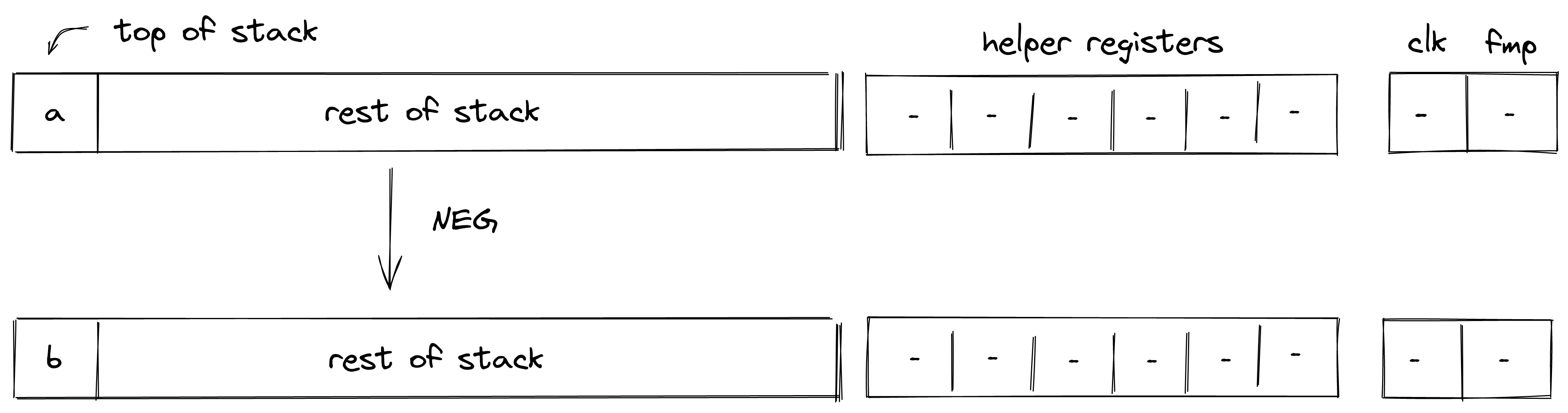
Stack transition for this operation must satisfy the following constraints:
The effect on the rest of the stack is:
- No change starting from position .
MUL
Assume and are the elements at the top of the stack. The MUL operation computes . The diagram below illustrates this graphically.
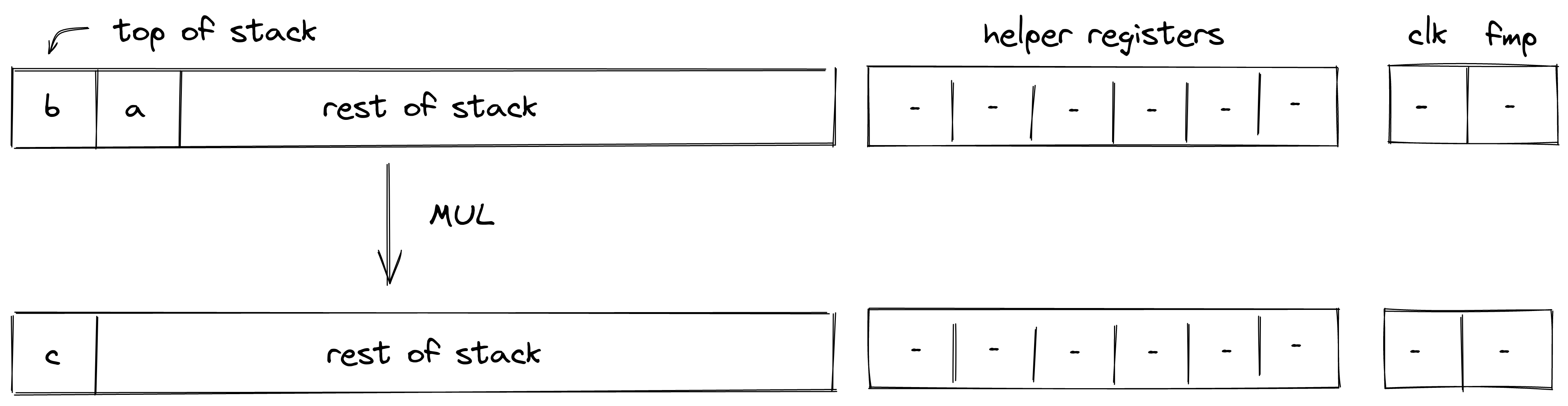
Stack transition for this operation must satisfy the following constraints:
The effect on the rest of the stack is:
- Left shift starting from position .
INV
Assume is the element at the top of the stack. The INV operation computes . The diagram below illustrates this graphically.
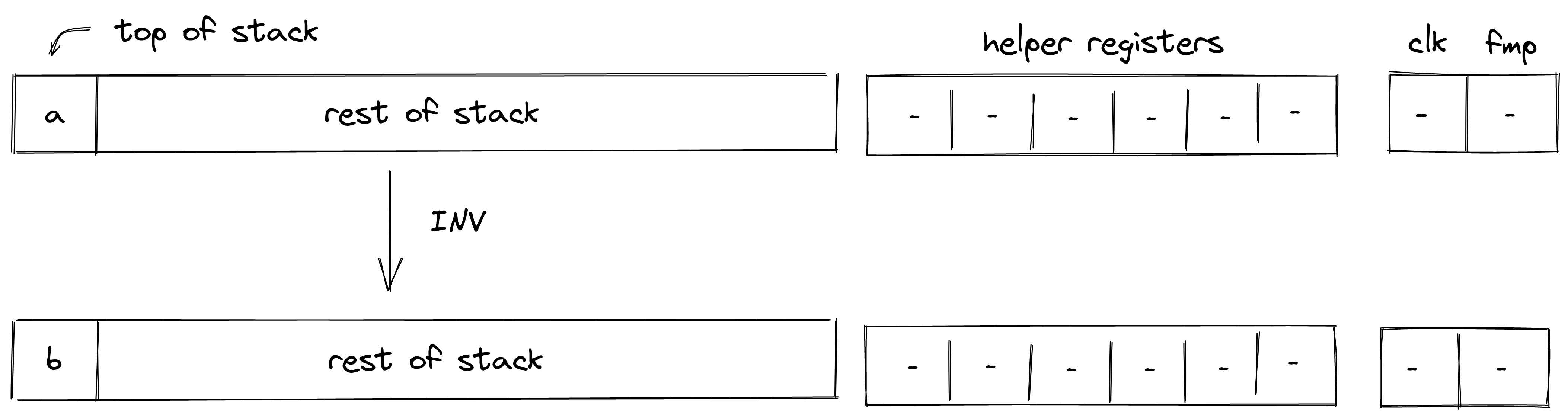
Stack transition for this operation must satisfy the following constraints:
Note that the above constraint can be satisfied only if the value in .
The effect on the rest of the stack is:
- No change starting from position .
INCR
Assume is the element at the top of the stack. The INCR operation computes . The diagram below illustrates this graphically.
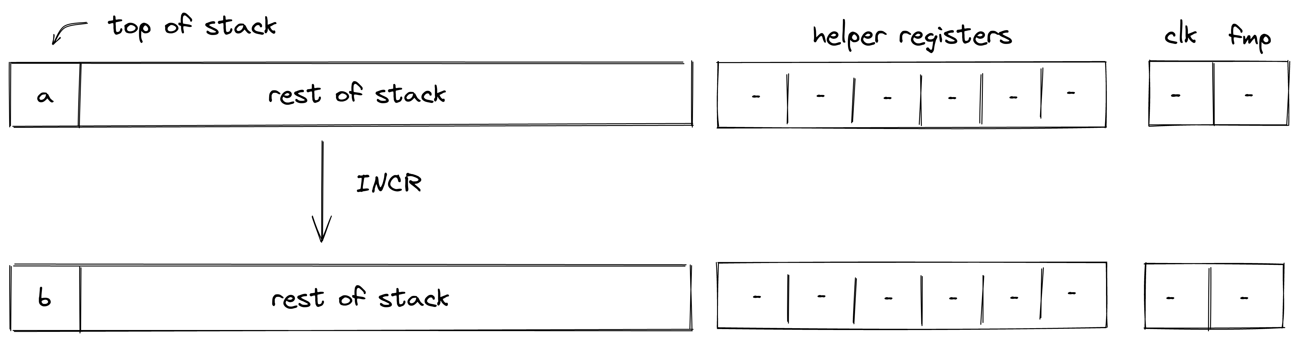
Stack transition for this operation must satisfy the following constraints:
The effect on the rest of the stack is:
- No change starting from position .
NOT
Assume is a binary value at the top of the stack. The NOT operation computes . The diagram below illustrates this graphically.
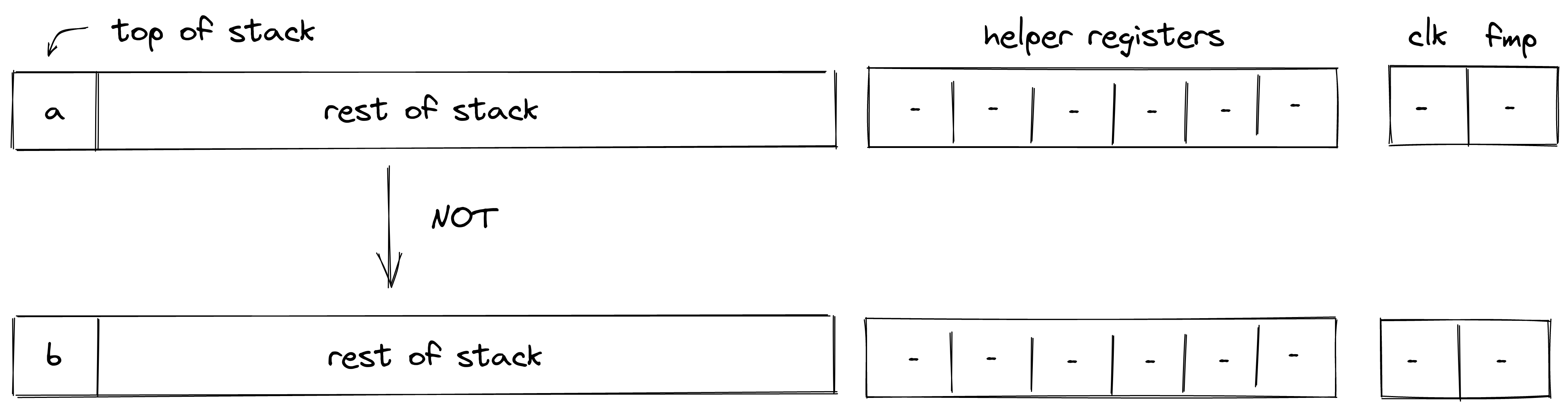
Stack transition for this operation must satisfy the following constraints:
The first constraint ensures that the value in is binary, and the second constraint ensures the correctness of the boolean NOT operation.
The effect on the rest of the stack is:
- No change starting from position .
AND
Assume and are binary values at the top of the stack. The AND operation computes . The diagram below illustrates this graphically.
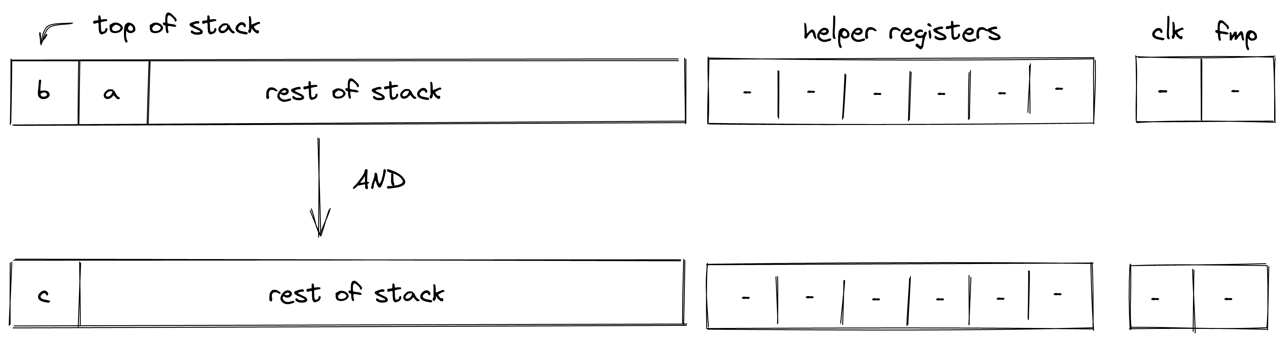
Stack transition for this operation must satisfy the following constraints:
The first two constraints ensure that the value in and are binary, and the third constraint ensures the correctness of the boolean AND operation.
The effect on the rest of the stack is:
- Left shift starting from position .
OR
Assume and are binary values at the top of the stack. The OR operation computes The diagram below illustrates this graphically.
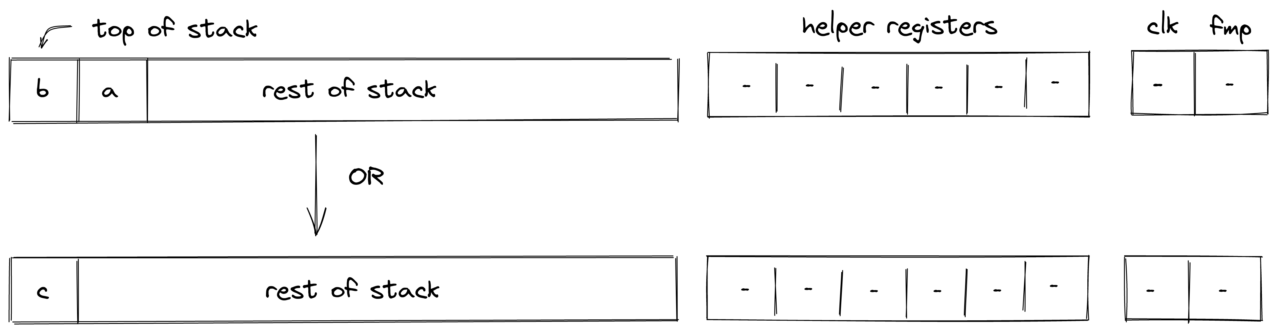
Stack transition for this operation must satisfy the following constraints:
The first two constraints ensure that the value in and are binary, and the third constraint ensures the correctness of the boolean OR operation.
The effect on the rest of the stack is:
- Left shift starting from position .
EQ
Assume and are the elements at the top of the stack. The EQ operation computes such that if , and otherwise. The diagram below illustrates this graphically.
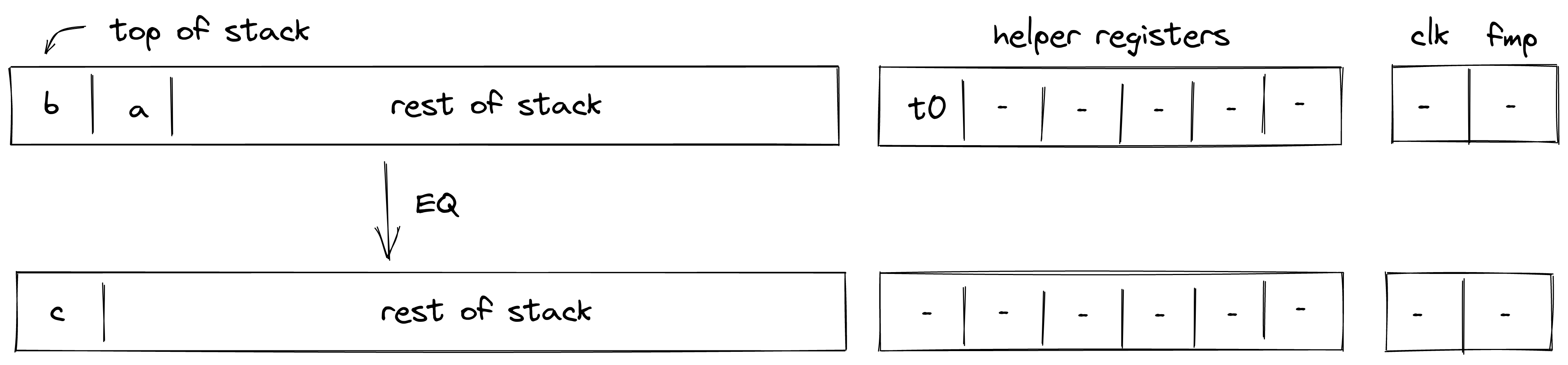
Stack transition for this operation must satisfy the following constraints:
To satisfy the above constraints, the prover must populate the value of helper register as follows:
- If , set .
- Otherwise, set to any value (e.g., ).
The effect on the rest of the stack is:
- Left shift starting from position .
EQZ
Assume is the element at the top of the stack. The EQZ operation computes such that if , and otherwise. The diagram below illustrates this graphically.
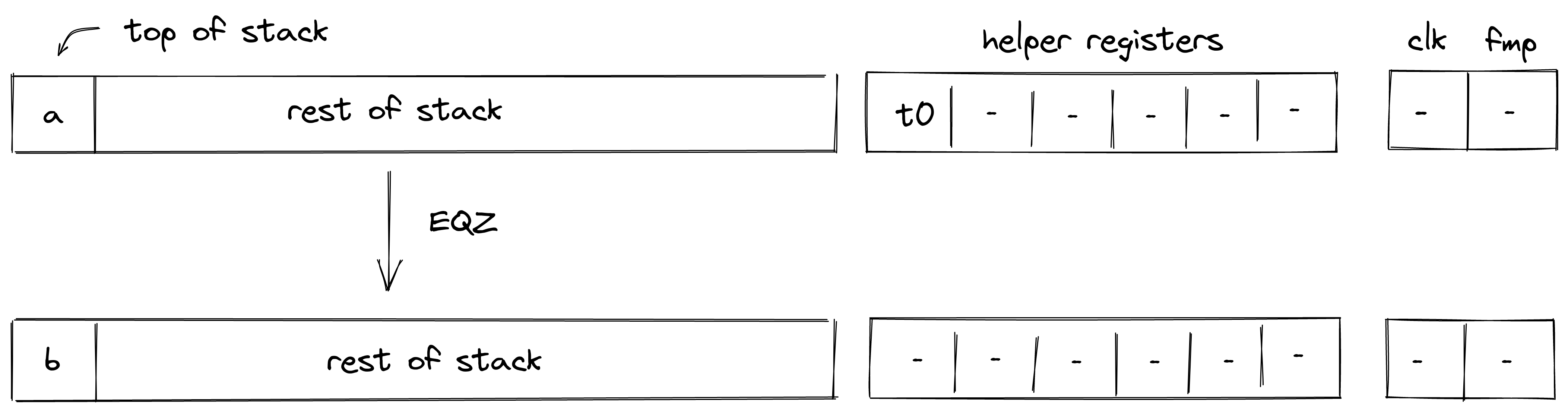
Stack transition for this operation must satisfy the following constraints:
To satisfy the above constraints, the prover must populate the value of helper register as follows:
- If , set .
- Otherwise, set to any value (e.g., ).
The effect on the rest of the stack is:
- No change starting from position .
EXPACC
The EXPACC operation computes one round of the expression . It is expected that Expacc is called at least num_exp_bits times, where num_exp_bits is the number of bits required to represent exp.
It pops elements from the top of the stack, performs a single round of exponent aggregation, and pushes the resulting values onto the stack. The diagram below illustrates this graphically.
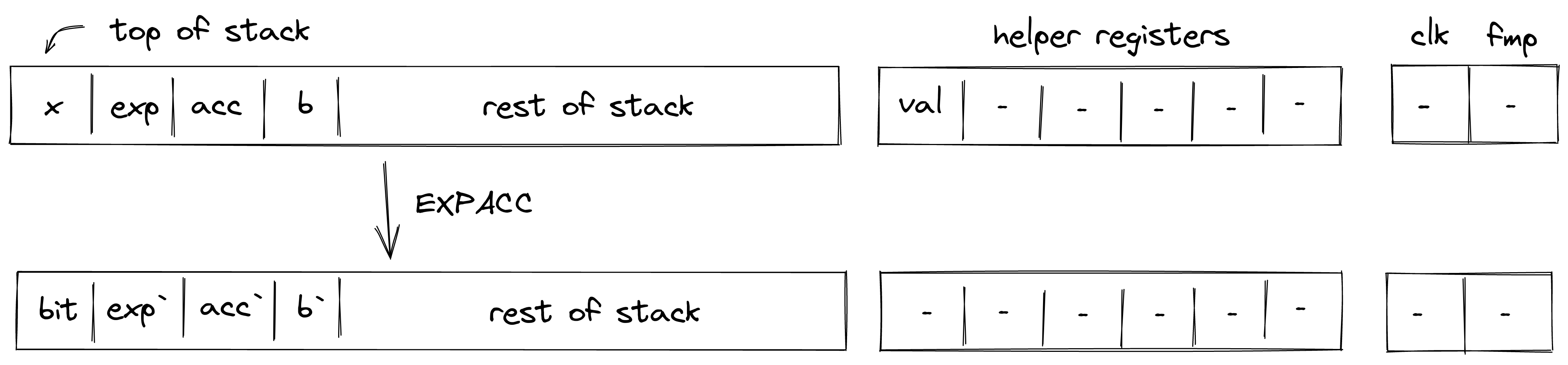
Expacc is based on the observation that the exponentiation of a number can be computed by repeatedly squaring the base and multiplying those powers of the base by the accumulator, for the powers of the base which correspond to the exponent's bits which are set to 1.
For example, take . Over the course of 3 iterations ( is in binary), the algorithm will compute , and (placed in base_acc). Hence, we want to multiply base_acc in acc when and when , which occurs on the first and third iterations (corresponding to the bits in the binary representation of 5).
Stack transition for this operation must satisfy the following constraints:
bit' should be a binary.
The base in the next frame should be the square of the base in the current frame.
The value val in the helper register is computed correctly using the bit and exp in next and current frame respectively.
The acc in the next frame is the product of val and acc in the current frame.
exp in the next frame is half of exp in the current frame (accounting for even/odd).
The effect on the rest of the stack is:
- No change starting from position .
EXT2MUL
The EXT2MUL operation pops top values from the top of the stack, performs multiplication between the two extension field elements, and pushes the resulting values onto the stack. The diagram below illustrates this graphically.
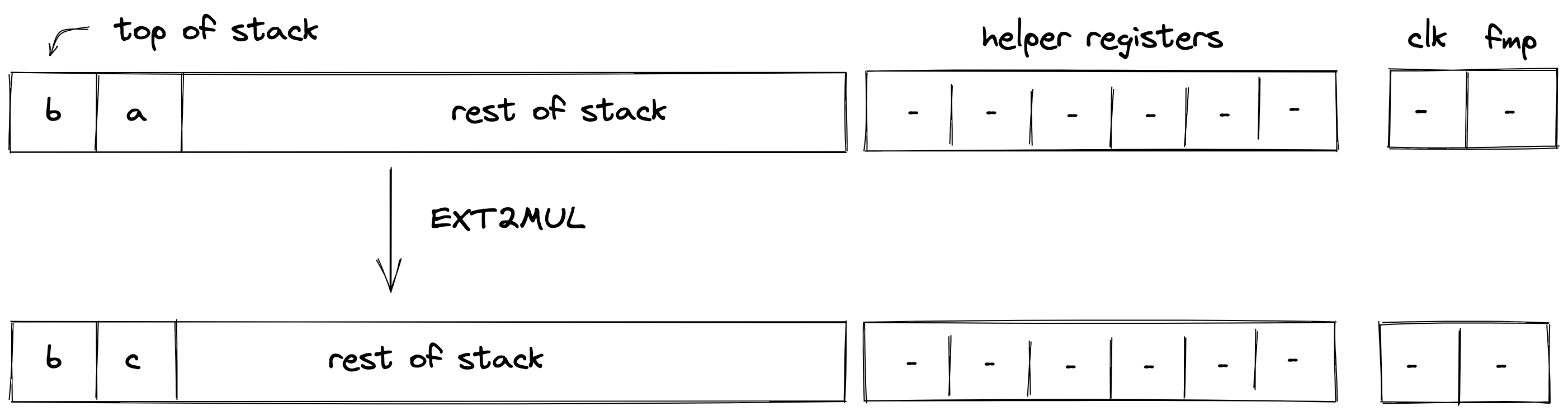
Stack transition for this operation must satisfy the following constraints:
The first stack element should be unchanged in the next frame.
The second stack element should be unchanged in the next frame.
The third stack element should satisfy the following constraint.
The fourth stack element should satisfy the following constraint.
The effect on the rest of the stack is:
- No change starting from position .
u32 Operations
In this section we describe semantics and AIR constraints of operations over u32 values (i.e., 32-bit unsigned integers) as they are implemented in Miden VM.
Range checks
Most operations described below require some number of 16-bit range checks (i.e., verifying that the value of a field element is smaller than ). The number of required range checks varies between and , depending on the operation. However, to simplify the constraint system, we force each relevant operation to consume exactly range checks.
To perform these range checks, the prover puts the values to be range-checked into helper registers , and then updates the range checker bus column according to the LogUp construction described in the range checker documentation, using multiplicity for each value.
This operation is enforced via the following constraint. Note that since constraints cannot include divisions, the actual constraint which is enforced will be expressed equivalently with all denominators multiplied through, resulting in a constraint of degree 5.
The above is just a partial constraint as it does not show the range checker's part of the constraint, which adds the required values into the bus column. It also omits the selector flag which is used to turn this constraint on only when executing relevant operations.
Checking element validity
Another primitive which is required by most of the operations described below is checking whether four 16-bit values form a valid field element. Assume , , , and are known to be 16-bit values, and we want to verify that is a valid field element.
For simplicity, let's denote:
We can then impose the following constraint to verify element validity:
Where is a value set non-deterministically by the prover.
The above constraint should hold only if either of the following hold:
To satisfy the latter equation, the prover needs to set , which is possible only when .
This constraint is sufficient because modulus in binary representation is 32 ones, followed by 31 zeros, followed by a single one:
This implies that the largest possible 64-bit value encoding a valid field element would be 32 ones, followed by 32 zeros:
Thus, for a 64-bit value to encode a valid field element, either the lower 32 bits must be all zeros, or the upper 32 bits must not be all ones (which is ).
U32SPLIT
Assume is the element at the top of the stack. The U32SPLIT operation computes , where contains the lower 32 bits of , and contains the upper 32 bits of . The diagram below illustrates this graphically.
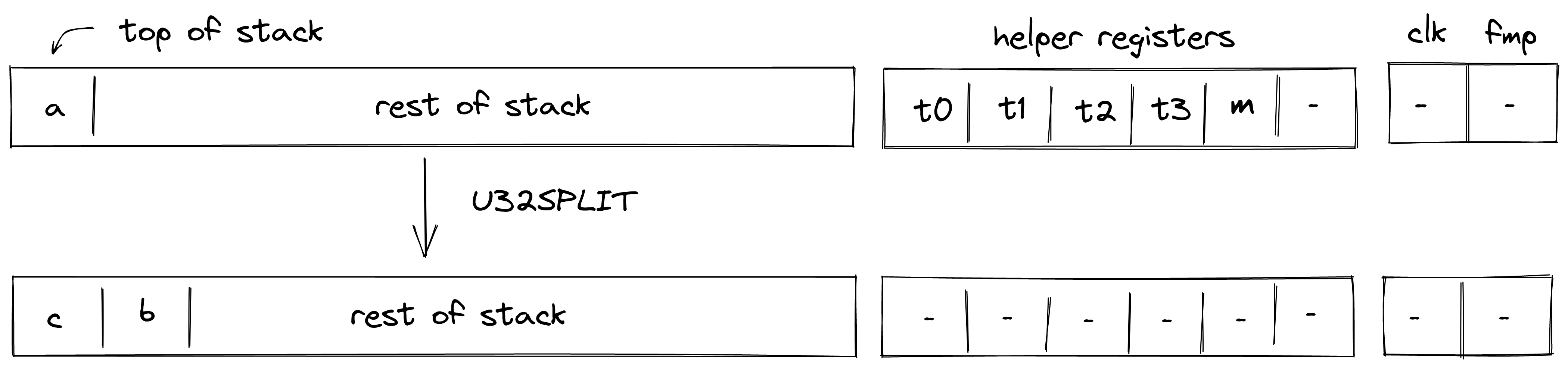
To facilitate this operation, the prover sets values in to 16-bit limbs of with being the least significant limb. Thus, stack transition for this operation must satisfy the following constraints:
In addition to the above constraints, we also need to verify that values in are smaller than , which we can do using 16-bit range checks as described previously. Also, we need to make sure that values in , when combined, form a valid field element, which we can do by putting a nondeterministic value into helper register and using the technique described here.
The effect of this operation on the rest of the stack is:
- Right shift starting from position .
U32ASSERT2
Assume and are the elements at the top of the stack. The U32ASSERT2 verifies that both and are smaller than . The diagram below illustrates this graphically.
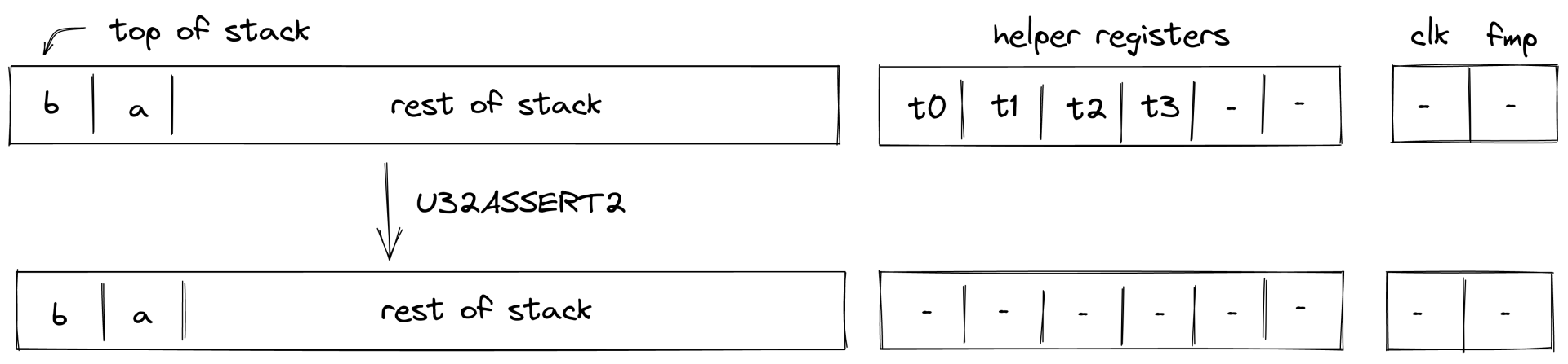
To facilitate this operation, the prover sets values in and to low and high 16-bit limbs of , and values in and to to low and high 16-bit limbs of . Thus, stack transition for this operation must satisfy the following constraints:
In addition to the above constraints, we also need to verify that values in are smaller than , which we can do using 16-bit range checks as described previously.
The effect of this operation on the rest of the stack is:
- No change starting from position - i.e., the state of the stack does not change.
U32ADD
Assume and are the values at the top of the stack which are known to be smaller than . The U32ADD operation computes , where contains the low 32-bits of the result, and is the carry bit. The diagram below illustrates this graphically.
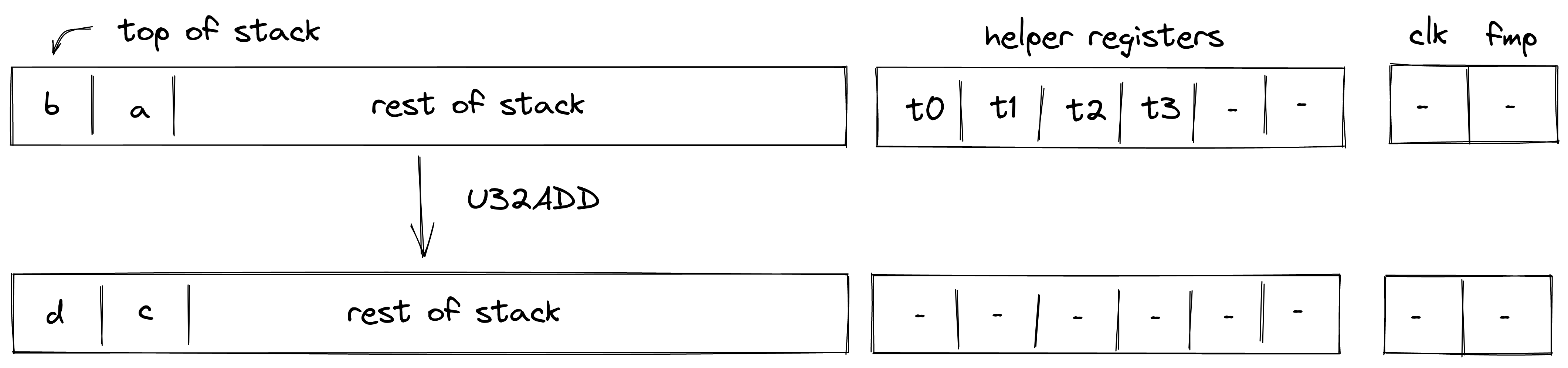
To facilitate this operation, the prover sets values in , , and to 16-bit limbs of with being the least significant limb. Value in is set to . Thus, stack transition for this operation must satisfy the following constraints:
In addition to the above constraints, we also need to verify that values in are smaller than , which we can do using 16-bit range checks as described previously.
The effect of this operation on the rest of the stack is:
- No change starting from position .
U32ADD3
Assume , , are the values at the top of the stack which are known to be smaller than . The U32ADD3 operation computes , where and contains the low and the high 32-bits of the result respectively. The diagram below illustrates this graphically.
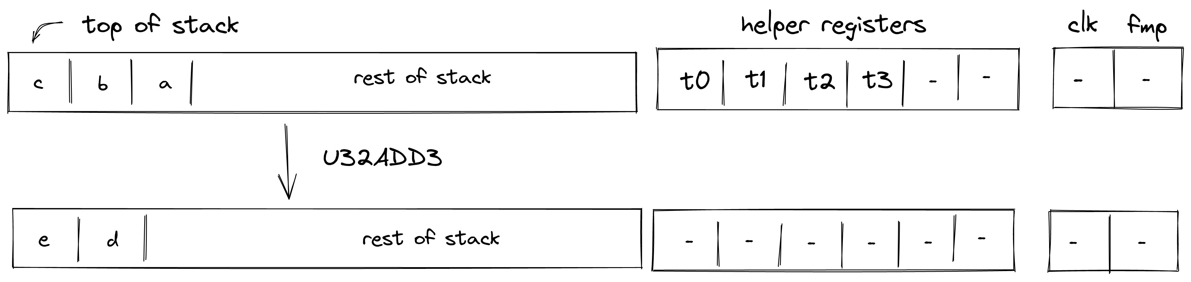
To facilitate this operation, the prover sets values in , , and to 16-bit limbs of with being the least significant limb. Value in is set to . Thus, stack transition for this operation must satisfy the following constraints:
In addition to the above constraints, we also need to verify that values in are smaller than , which we can do using 16-bit range checks as described previously.
The effect of this operation on the rest of the stack is:
- Left shift starting from position .
U32SUB
Assume and are the values at the top of the stack which are known to be smaller than . The U32SUB operation computes , where contains the 32-bit result in two's complement, and is the borrow bit. The diagram below illustrates this graphically.
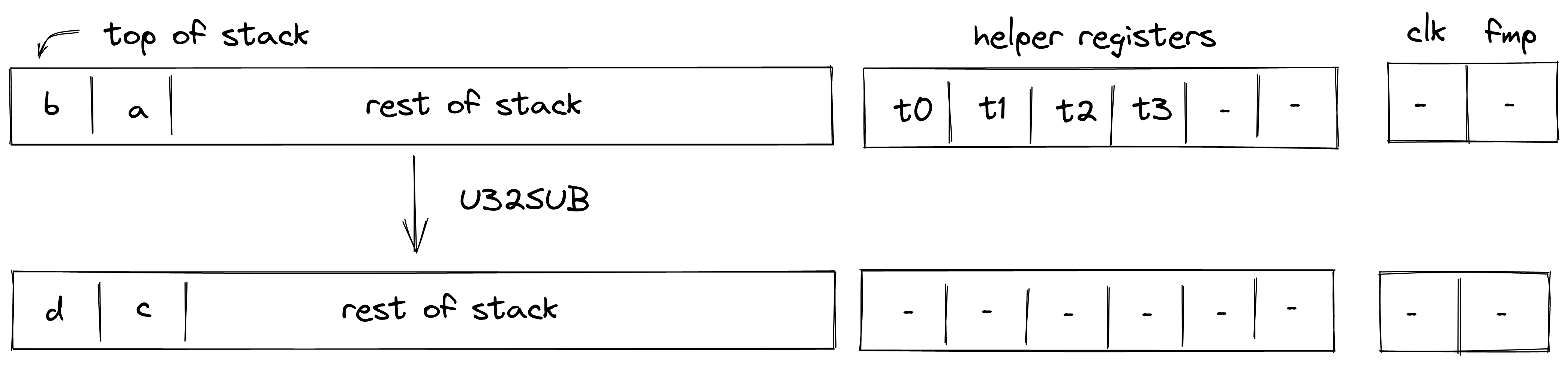
To facilitate this operation, the prover sets values in and to the low and the high 16-bit limbs of respectively. Values in and are set to . Thus, stack transition for this operation must satisfy the following constraints:
In addition to the above constraints, we also need to verify that values in are smaller than , which we can do using 16-bit range checks as described previously.
The effect of this operation on the rest of the stack is:
- No change starting from position .
U32MUL
Assume and are the values at the top of the stack which are known to be smaller than . The U32MUL operation computes , where and contain the low and the high 32-bits of the result respectively. The diagram below illustrates this graphically.
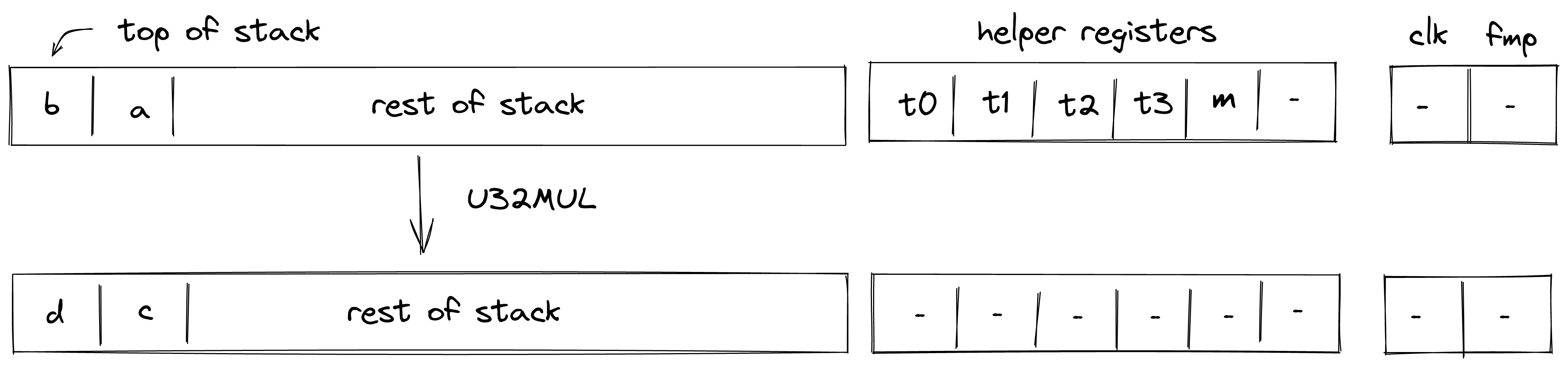
To facilitate this operation, the prover sets values in to 16-bit limbs of with being the least significant limb. Thus, stack transition for this operation must satisfy the following constraints:
In addition to the above constraints, we also need to verify that values in are smaller than , which we can do using 16-bit range checks as described previously. Also, we need to make sure that values in , when combined, form a valid field element, which we can do by putting a nondeterministic value into helper register and using the technique described here.
The effect of this operation on the rest of the stack is:
- No change starting from position .
U32MADD
Assume , , are the values at the top of the stack which are known to be smaller than . The U32MADD operation computes , where and contains the low and the high 32-bits of . The diagram below illustrates this graphically.
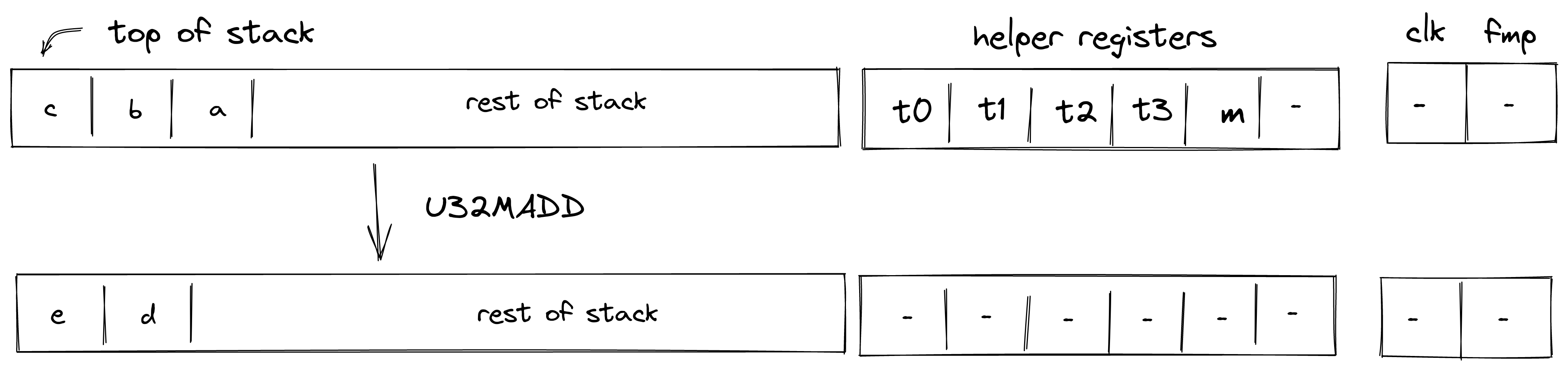
To facilitate this operation, the prover sets values in to 16-bit limbs of with being the least significant limb. Thus, stack transition for this operation must satisfy the following constraints:
In addition to the above constraints, we also need to verify that values in are smaller than , which we can do using 16-bit range checks as described previously. Also, we need to make sure that values in , when combined, form a valid field element, which we can do by putting a nondeterministic value into helper register and using the technique described here.
Note: that the above constraints guarantee the correctness of the operation iff cannot overflow field modules (which is the case for the field with modulus ).
The effect of this operation on the rest of the stack is:
- Left shift starting from position .
U32DIV
Assume and are the values at the top of the stack which are known to be smaller than . The U32DIV operation computes , where contains the quotient and contains the remainder. The diagram below illustrates this graphically.
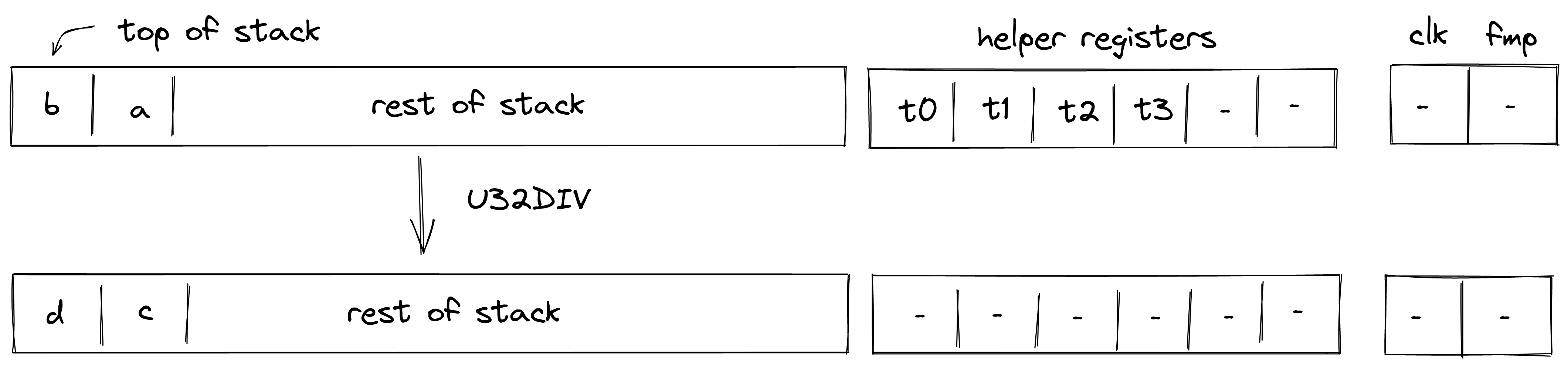
To facilitate this operation, the prover sets values in and to 16-bit limbs of , and values in and to 16-bit limbs of . Thus, stack transition for this operation must satisfy the following constraints:
The second constraint enforces that , while the third constraint enforces that .
The effect of this operation on the rest of the stack is:
- No change starting from position .
U32AND
Assume and are the values at the top of the stack. The U32AND operation computes , where is the result of performing a bitwise AND on and . The diagram below illustrates this graphically.
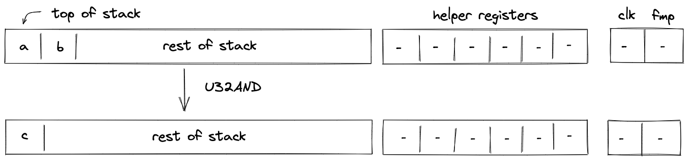
To facilitate this operation, we will need to make a request to the chiplet bus by dividing its current value by the value representing bitwise operation request. This can be enforced with the following constraint:
In the above, is the unique operation label of the bitwise AND operation.
Note: unlike for many other u32 operations, bitwise AND operation does not assume that the values at the top of the stack are smaller than . This is because the lookup will fail for any inputs which are not 32-bit integers.
The effect of this operation on the rest of the stack is:
- Left shift starting from position .
U32XOR
Assume and are the values at the top of the stack. The U32XOR operation computes , where is the result of performing a bitwise XOR on and . The diagram below illustrates this graphically.
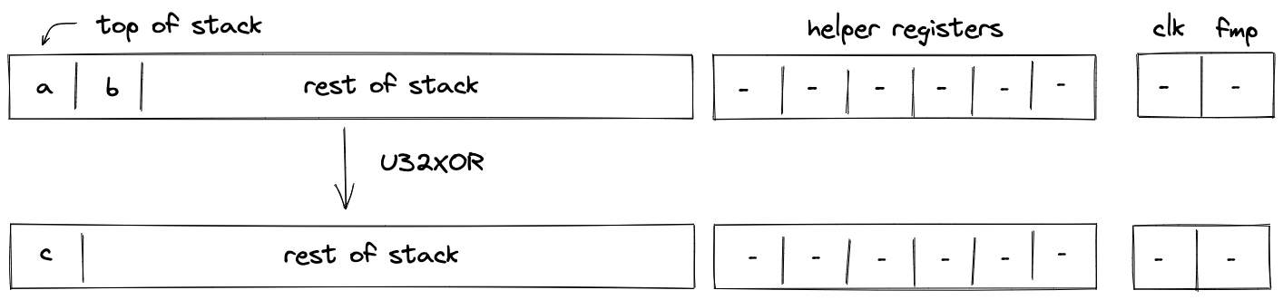
To facilitate this operation, we will need to make a request to the chiplet bus by dividing its current value by the value representing bitwise operation request. This can be enforced with the following constraint:
In the above, is the unique operation label of the bitwise XOR operation.
Note: unlike for many other u32 operations, bitwise XOR operation does not assume that the values at the top of the stack are smaller than . This is because the lookup will fail for any inputs which are not 32-bit integers.
The effect of this operation on the rest of the stack is:
- Left shift starting from position .
Stack Manipulation
In this section we describe the AIR constraints for Miden VM stack manipulation operations.
PAD
The PAD operation pushes a onto the stack. The diagram below illustrates this graphically.
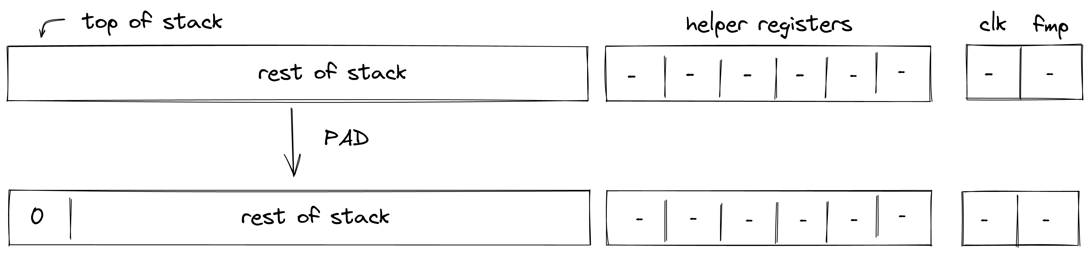
Stack transition for this operation must satisfy the following constraints:
The effect of this operation on the rest of the stack is:
- Right shift starting from position .
DROP
The DROP operation removes an element from the top of the stack. The diagram below illustrates this graphically.
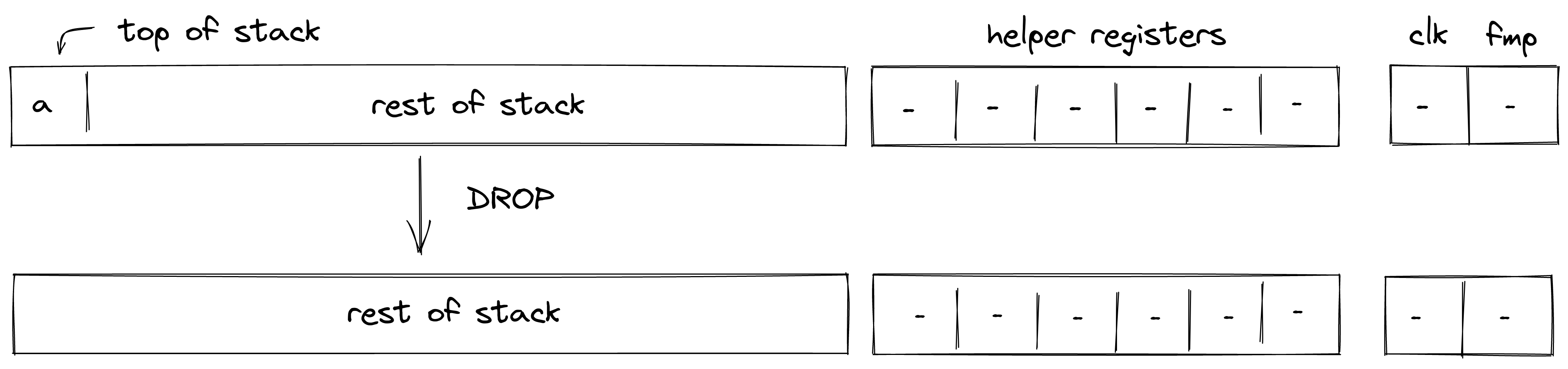
The DROP operation shifts the stack by element to the left, but does not impose any additional constraints. The degree of left shift constraints is .
The effect of this operation on the rest of the stack is:
- Left shift starting from position .
DUP(n)
The DUP(n) operations push a copy of the -th stack element onto the stack. Eg. DUP (same as DUP0) pushes a copy of the top stack element onto the stack. Similarly, DUP5 pushes a copy of the -th stack element onto the stack. This operation is valid for . The diagram below illustrates this graphically.
.png)
Stack transition for this operation must satisfy the following constraints:
where is the depth of the stack from where the element has been copied.
The effect of this operation on the rest of the stack is:
- Right shift starting from position .
SWAP
The SWAP operations swaps the top two elements of the stack. The diagram below illustrates this graphically.
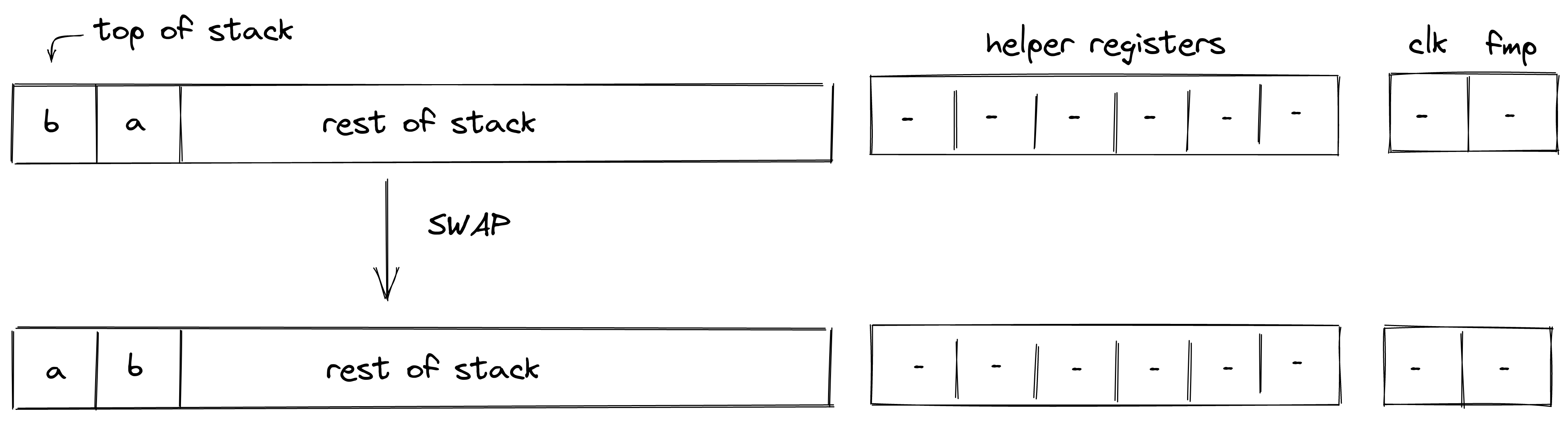
Stack transition for this operation must satisfy the following constraints:
The effect of this operation on the rest of the stack is:
- No change starting from position .
SWAPW
The SWAPW operation swaps stack elements with elements . The diagram below illustrates this graphically.
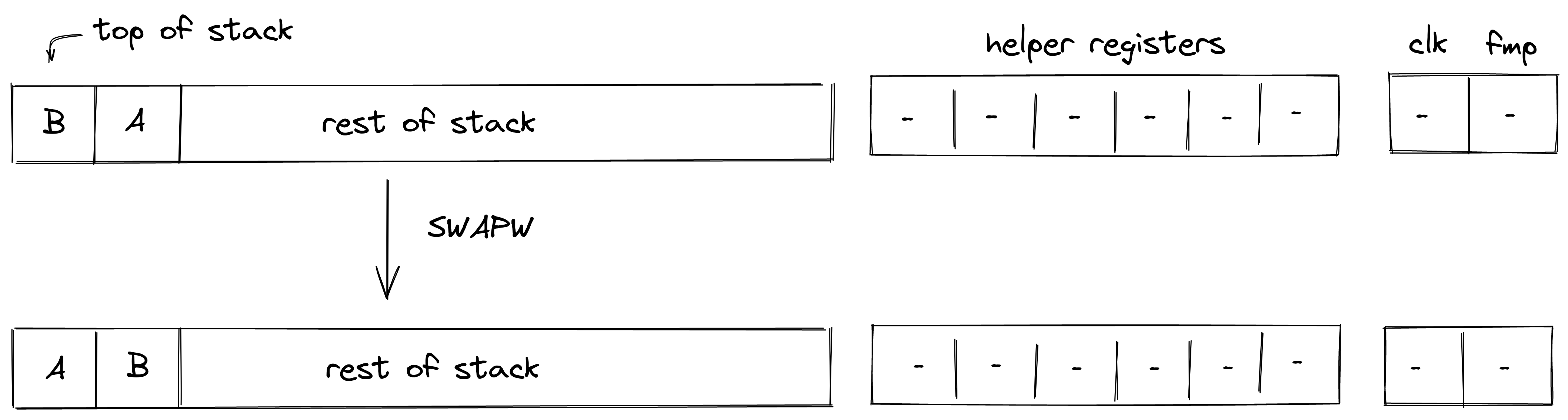
Stack transition for this operation must satisfy the following constraints:
The effect of this operation on the rest of the stack is:
- No change starting from position .
SWAPW2
The SWAPW2 operation swaps stack elements with elements . The diagram below illustrates this graphically.
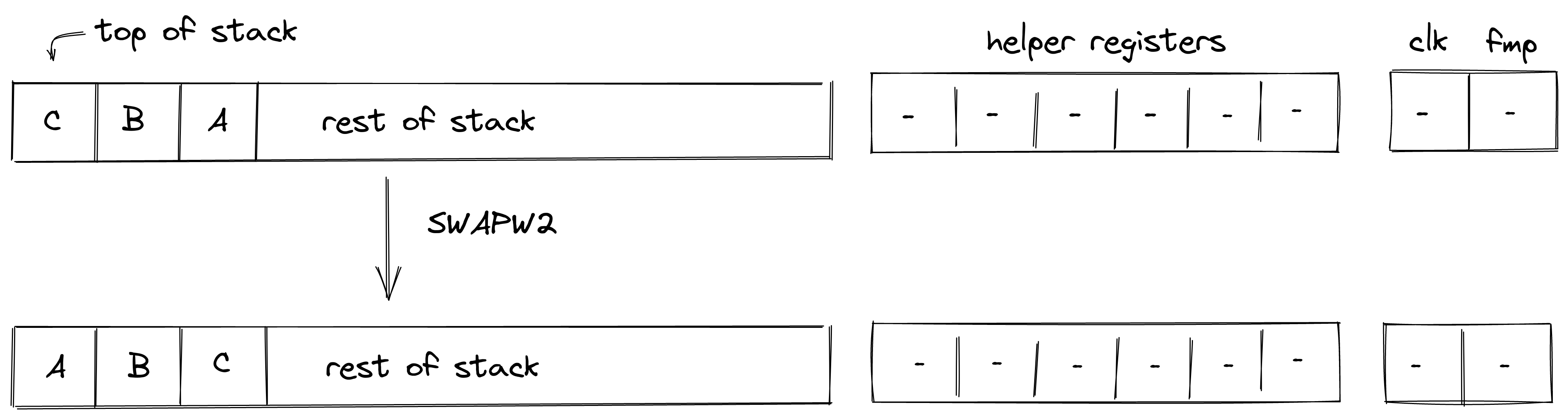
Stack transition for this operation must satisfy the following constraints:
The effect of this operation on the rest of the stack is:
- No change for elements .
- No change starting from position .
SWAPW3
The SWAPW3 operation swaps stack elements with elements . The diagram below illustrates this graphically.
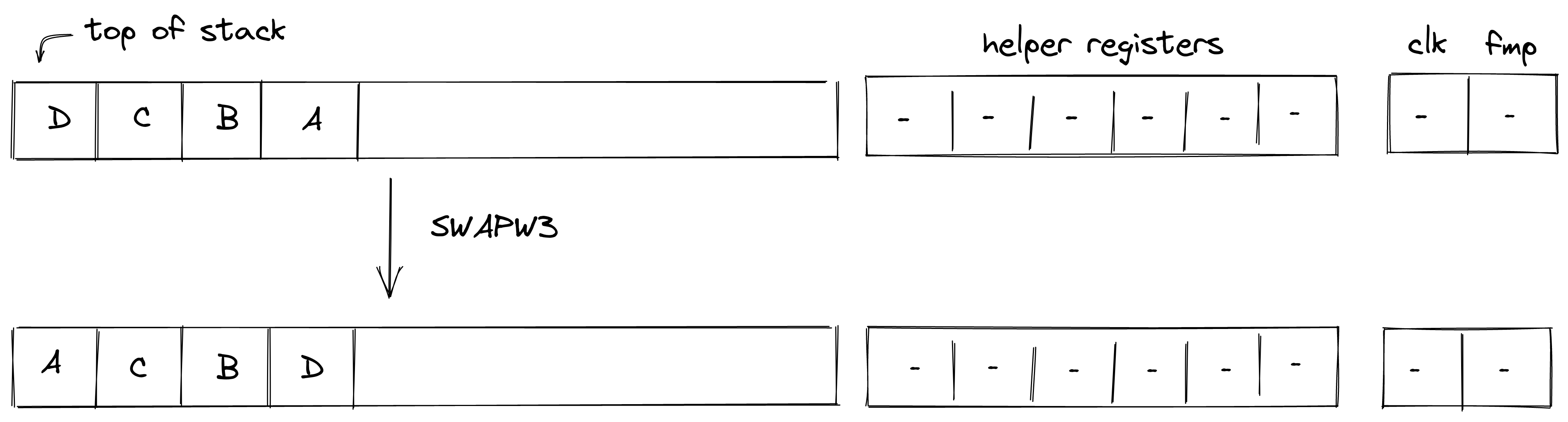
Stack transition for this operation must satisfy the following constraints:
The effect of this operation on the rest of the stack is:
- No change for elements .
- No change starting from position .
SWAPDW
The SWAPDW operation swaps stack elements with elements . The diagram below illustrates this graphically.
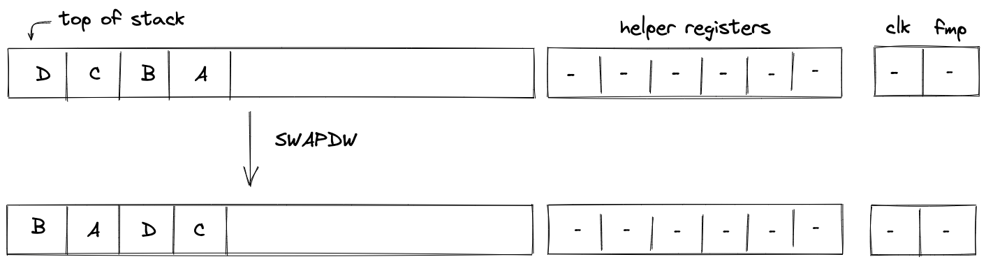
Stack transition for this operation must satisfy the following constraints:
The effect of this operation on the rest of the stack is:
- No change starting from position .
MOVUP(n)
The MOVUP(n) operation moves the -th element of the stack to the top of the stack. For example, MOVUP2 moves element at depth to the top of the stack. All elements with depth less than are shifted to the right by one, while elements with depth greater than remain in place, and the depth of the stack does not change. This operation is valid for . The diagram below illustrates this graphically.
.png)
Stack transition for this operation must satisfy the following constraints:
where is the depth of the element which is moved moved to the top of the stack.
The effect of this operation on the rest of the stack is:
- Right shift for elements between and .
- No change starting from position .
MOVDN(n)
The MOVDN(n) operation moves the top element of the stack to the -th position. For example, MOVDN2 moves the top element of the stack to depth . All the elements with depth less than are shifted to the left by one, while elements with depth greater than remain in place, and the depth of the stack does not change. This operation is valid for . The diagram below illustrates this graphically.
.png)
Stack transition for this operation must satisfy the following constraints:
where is the depth to which the top stack element is moved.
The effect of this operation on the rest of the stack is:
- Left shift for elements between and .
- No change starting from position .
CSWAP
The CSWAP operation pops an element off the stack and if the element is , swaps the top two remaining elements. If the popped element is , the rest of the stack remains unchanged. The diagram below illustrates this graphically.
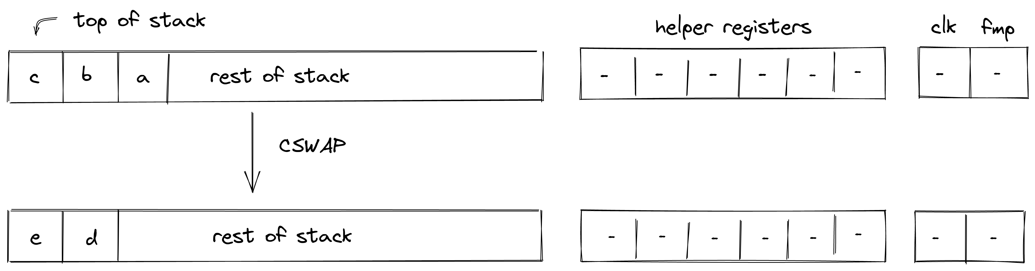
In the above:
Stack transition for this operation must satisfy the following constraints:
We also need to enforce that the value in is binary. This can be done with the following constraint:
The effect of this operation on the rest of the stack is:
- Left shift starting from position .
CSWAPW
The CSWAPW operation pops an element off the stack and if the element is , swaps elements with elements . If the popped element is , the rest of the stack remains unchanged. The diagram below illustrates this graphically.
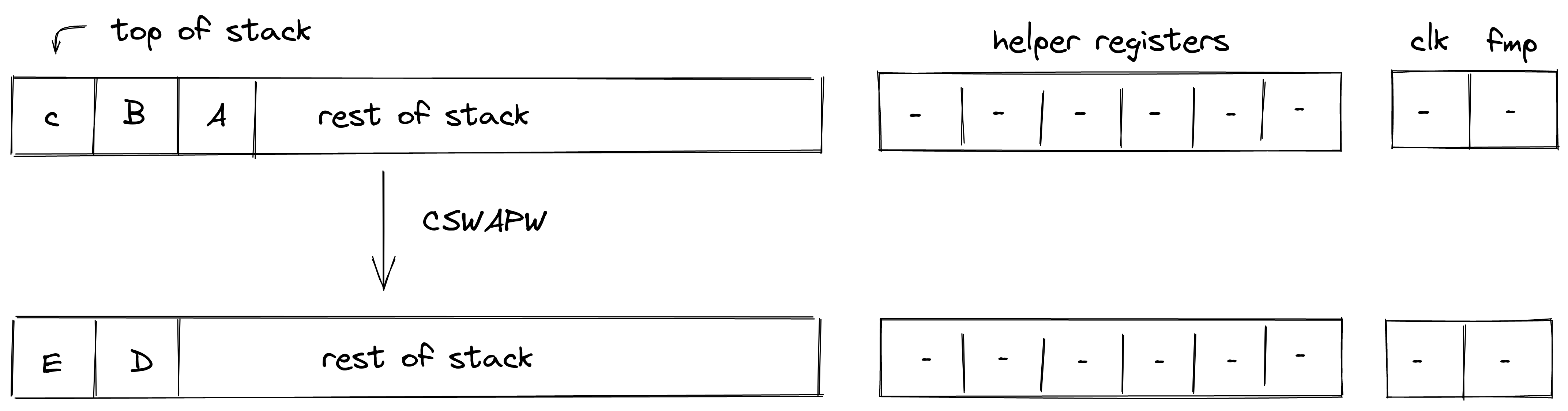
In the above:
Stack transition for this operation must satisfy the following constraints:
We also need to enforce that the value in is binary. This can be done with the following constraint:
The effect of this operation on the rest of the stack is:
- Left shift starting from position .
Input / output operations
In this section we describe the AIR constraints for Miden VM input / output operations. These operations move values between the stack and other components of the VM such as program code (i.e., decoder), memory, and advice provider.
PUSH
The PUSH operation pushes the provided immediate value onto the stack non-deterministically (i.e., sets the value of register); it is the responsibility of the Op Group Table to ensure that the correct value was pushed on the stack. The semantics of this operation are explained in the decoder section.
The effect of this operation on the rest of the stack is:
- Right shift starting from position .
SDEPTH
Assume is the current depth of the stack stored in the stack bookkeeping register (as described here). The SDEPTH pushes onto the stack. The diagram below illustrates this graphically.
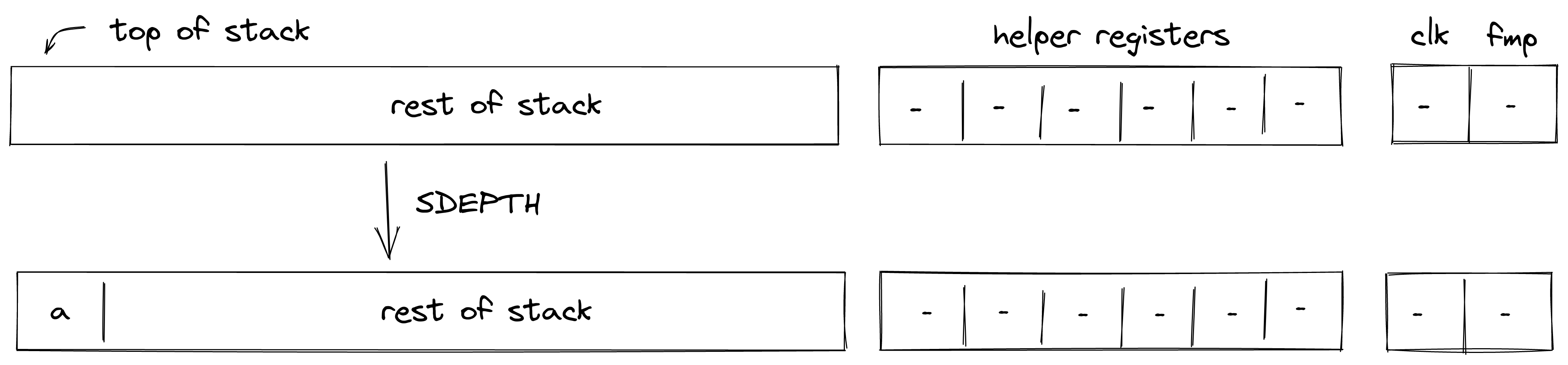
Stack transition for this operation must satisfy the following constraints:
The effect of this operation on the rest of the stack is:
- Right shift starting from position .
ADVPOP
Assume is an element at the top of the advice stack. The ADVPOP operation removes from the advice stack and pushes it onto the operand stack. The diagram below illustrates this graphically.
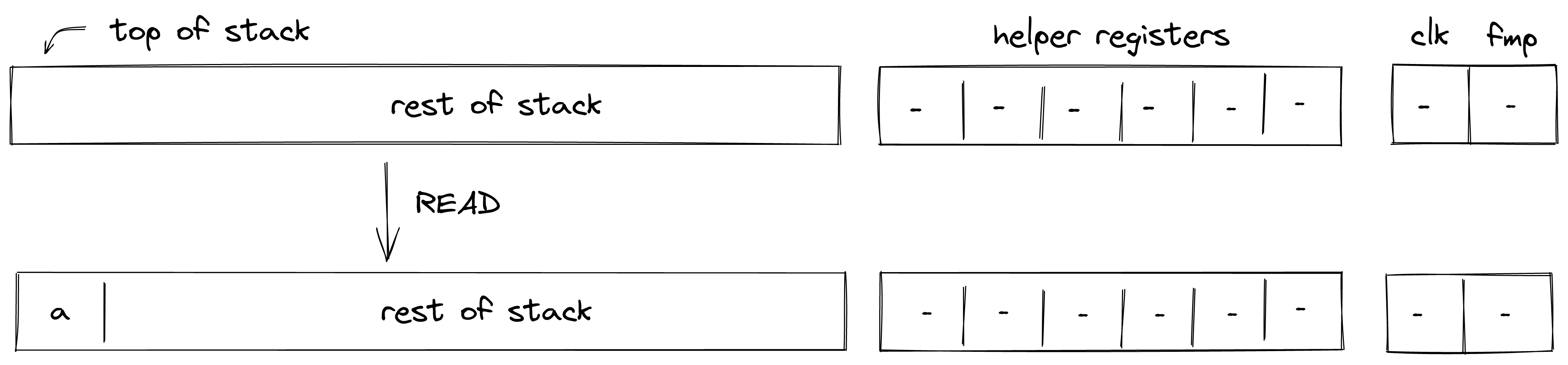
The ADVPOP operation does not impose any constraints against the first element of the operand stack.
The effect of this operation on the rest of the operand stack is:
- Right shift starting from position .
ADVPOPW
Assume , , , and , are the elements at the top of the advice stack (with being on top). The ADVPOPW operation removes these elements from the advice stack and puts them onto the operand stack by overwriting the top stack elements. The diagram below illustrates this graphically.
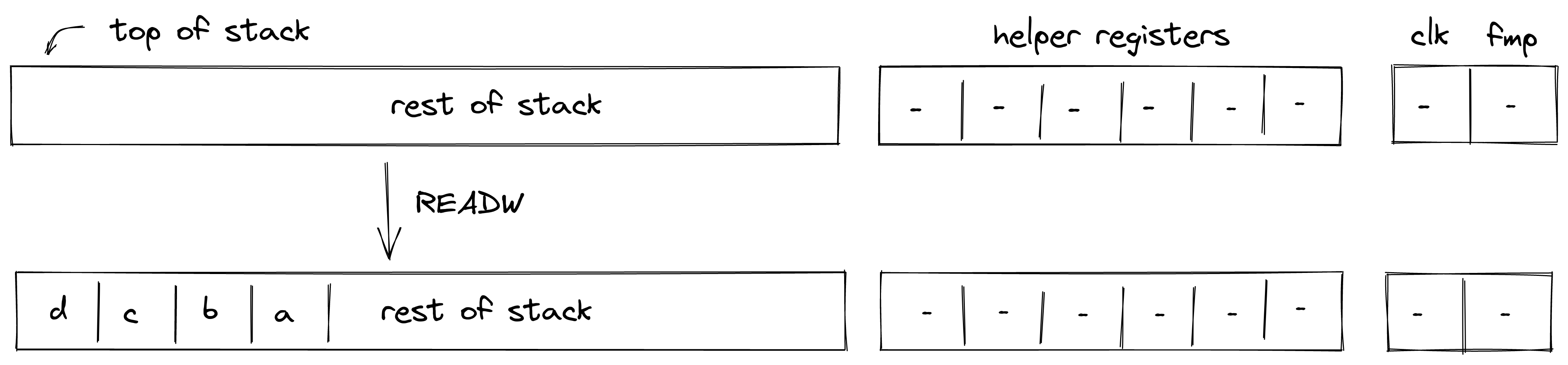
The ADVPOPW operation does not impose any constraints against the top elements of the operand stack.
The effect of this operation on the rest of the operand stack is:
- No change starting from position .
Memory access operations
Miden VM exposes several operations for reading from and writing to random access memory. Memory in Miden VM is managed by the Memory chiplet.
Communication between the stack and the memory chiplet is accomplished via the chiplet bus . To make requests to the chiplet bus we need to divide its current value by the value representing memory access request. The structure of memory access request value is described here.
To enforce the correctness of memory access, we can use the following constraint:
In the above, is the value of memory access request. Thus, to describe AIR constraint for memory operations, it is sufficient to describe how is computed. We do this in the following sections.
MLOADW
Assume that the word with elements is located in memory starting at address . The MLOADW operation pops an element off the stack, interprets it as a memory address, and replaces the remaining 4 elements at the top of the stack with values located at the specified address. The diagram below illustrates this graphically.
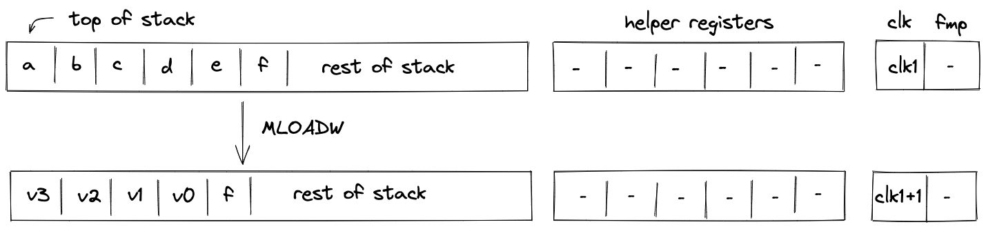
To simplify description of the memory access request value, we first define a variable for the value that represents the state of memory after the operation:
Using the above variable, we define the value representing the memory access request as follows:
In the above:
- is the unique operation label of the memory "read word" operation.
- is the identifier of the current memory context.
- is the memory address from which the values are to be loaded onto the stack.
- is the current clock cycle of the VM.
The effect of this operation on the rest of the stack is:
- Left shift starting from position .
MLOAD
Assume that the element is located in memory at address . The MLOAD operation pops an element off the stack, interprets it as a memory address, and pushes the element located at the specified address to the stack. The diagram below illustrates this graphically.
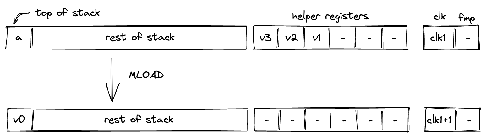
We define the value representing the memory access request as follows:
In the above:
- is the unique operation label of the memory "read element" operation.
- is the identifier of the current memory context.
- is the memory address from which the value is to be loaded onto the stack.
- is the current clock cycle of the VM.
The effect of this operation on the rest of the stack is:
- No change starting from position .
MSTOREW
The MSTOREW operation pops an element off the stack, interprets it as a memory address, and writes the remaining elements at the top of the stack into memory starting at the specified address. The stored elements are not removed from the stack. The diagram below illustrates this graphically.
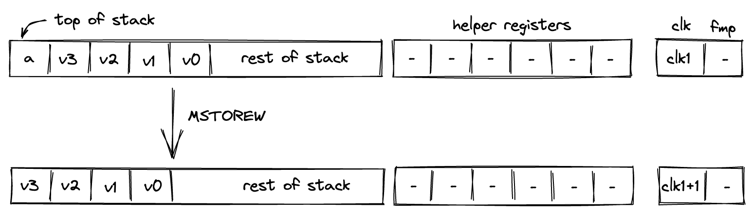
After the operation the contents of memory at addresses , , , would be set to , respectively.
To simplify description of the memory access request value, we first define a variable for the value that represents the state of memory after the operation:
Using the above variable, we define the value representing the memory access request as follows:
In the above:
- is the unique operation label of the memory "write word" operation.
- is the identifier of the current memory context.
- is the memory address into which the values from the stack are to be saved.
- is the current clock cycle of the VM.
The effect of this operation on the rest of the stack is:
- Left shift starting from position .
MSTORE
The MSTORE operation pops an element off the stack, interprets it as a memory address, and writes the remaining element at the top of the stack into memory at the specified memory address. The diagram below illustrates this graphically.
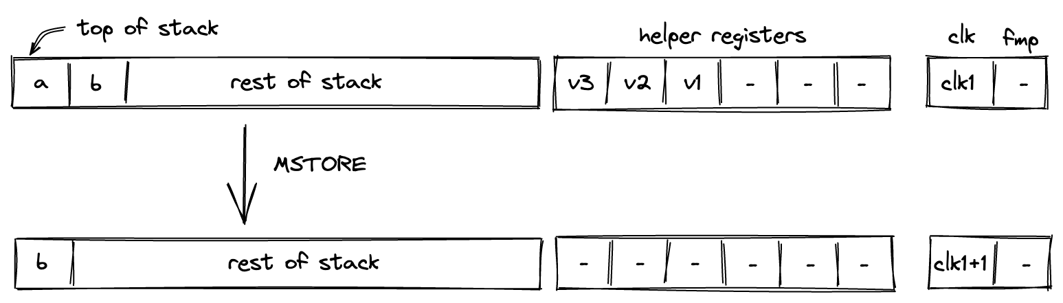
After the operation the contents of memory at address would be set to .
We define the value representing the memory access request as follows:
In the above:
- is the unique operation label of the memory "write element" operation.
- is the identifier of the current memory context.
- is the memory address into which the value from the stack is to be saved.
- is the current clock cycle of the VM.
The effect of this operation on the rest of the stack is:
- Left shift starting from position .
MSTREAM
The MSTREAM operation loads two words from memory, and replaces the top 8 elements of the stack with them, element-wise, in stack order. The start memory address from which the words are loaded is stored in the 13th stack element (position 12). The diagram below illustrates this graphically.
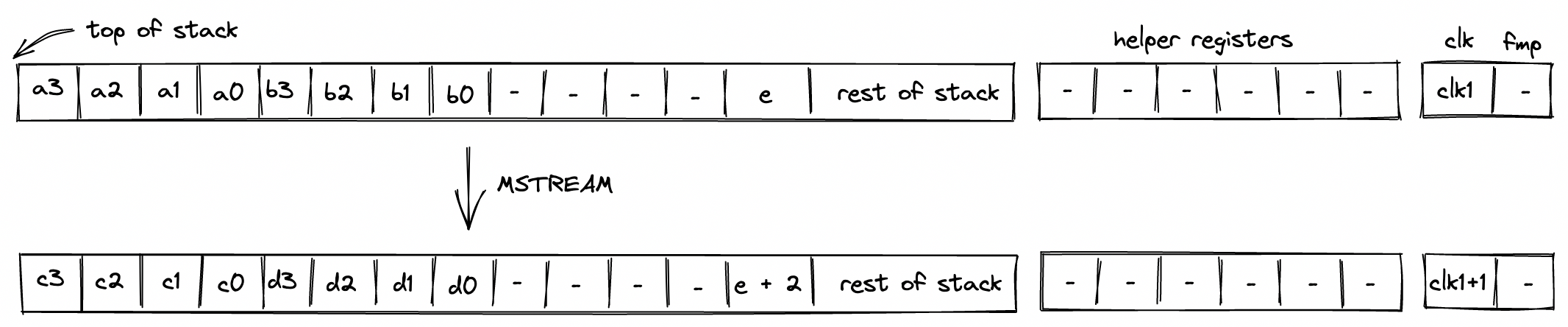
After the operation, the memory address is incremented by 8.
To simplify description of the memory access request value, we first define variables for the values that represent the state of memory after the operation:
Using the above variables, we define the values representing the memory access request as follows:
In the above:
- is the unique operation label of the memory "read word" operation.
- is the identifier of the current memory context.
- and are the memory addresses from which the words are to be loaded onto the stack.
- is the current clock cycle of the VM.
The effect of this operation on the rest of the stack is:
- No change starting from position except position .
Cryptographic operations
In this section we describe the AIR constraints for Miden VM cryptographic operations.
Cryptographic operations in Miden VM are performed by the Hash chiplet. Communication between the stack and the hash chiplet is accomplished via the chiplet bus . To make requests to and to read results from the chiplet bus we need to divide its current value by the value representing the request.
Thus, to describe AIR constraints for the cryptographic operations, we need to define how to compute these input and output values within the stack. We do this in the following sections.
HPERM
The HPERM operation applies Rescue Prime Optimized permutation to the top elements of the stack. The stack is assumed to be arranged so that the elements of the rate are at the top of the stack. The capacity word follows, with the number of elements to be hashed at the deepest position in stack. The diagram below illustrates this graphically.
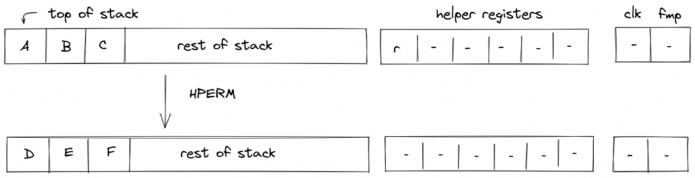
In the above, (located in the helper register ) is the row address from the hash chiplet set by the prover non-deterministically.
For the HPERM operation, we define input and output values as follows:
In the above, and are the unique operation labels for initiating a linear hash and reading the full state of the hasher respectively. Also note that the term for is missing from the above expressions because for Rescue Prime Optimized permutation computation the index column is expected to be set to .
Using the above values, we can describe the constraint for the chiplet bus column as follows:
The above constraint enforces that the specified input and output rows must be present in the trace of the hash chiplet, and that they must be exactly rows apart.
The effect of this operation on the rest of the stack is:
- No change starting from position .
MPVERIFY
The MPVERIFY operation verifies that a Merkle path from the specified node resolves to the specified root. This operation can be used to prove that the prover knows a path in the specified Merkle tree which starts with the specified node.
Prior to the operation, the stack is expected to be arranged as follows (from the top):
- Value of the node, 4 elements ( in the below image)
- Depth of the path, 1 element ( in the below image)
- Index of the node, 1 element ( in the below image)
- Root of the tree, 4 elements ( in the below image)
The Merkle path itself is expected to be provided by the prover non-deterministically (via the advice provider). If the prover is not able to provide the required path, the operation fails. Otherwise, the state of the stack does not change. The diagram below illustrates this graphically.
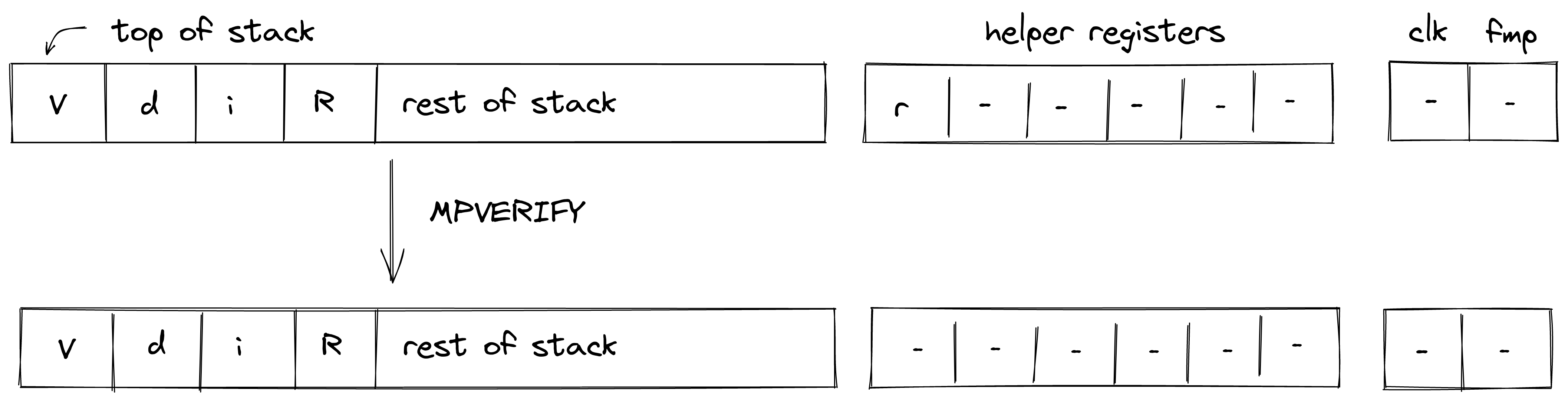
In the above, (located in the helper register ) is the row address from the hash chiplet set by the prover non-deterministically.
For the MPVERIFY operation, we define input and output values as follows:
In the above, and are the unique operation labels for initiating a Merkle path verification computation and reading the hash result respectively. The sum expression for inputs computes the value of the leaf node, while the sum expression for the output computes the value of the tree root.
Using the above values, we can describe the constraint for the chiplet bus column as follows:
The above constraint enforces that the specified input and output rows must be present in the trace of the hash chiplet, and that they must be exactly rows apart, where is the depth of the node.
The effect of this operation on the rest of the stack is:
- No change starting from position .
MRUPDATE
The MRUPDATE operation computes a new root of a Merkle tree where a node at the specified position is updated to the specified value.
The stack is expected to be arranged as follows (from the top):
- old value of the node, 4 element ( in the below image)
- depth of the node, 1 element ( in the below image)
- index of the node, 1 element ( in the below image)
- current root of the tree, 4 elements ( in the below image)
- new value of the node, 4 element ( in the below image)
The Merkle path for the node is expected to be provided by the prover non-deterministically (via merkle sets). At the end of the operation, the old node value is replaced with the new root value computed based on the provided path. Everything else on the stack remains the same. The diagram below illustrates this graphically.
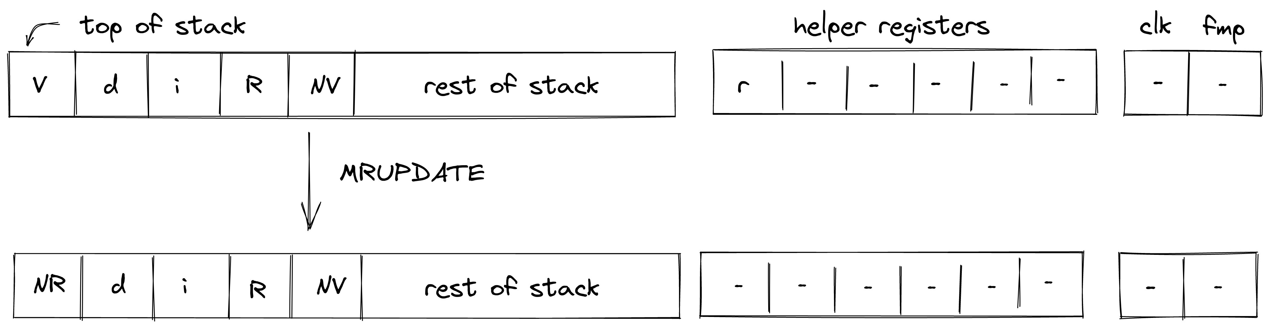
In the above, (located in the helper register ) is the row address from the hash chiplet set by the prover non-deterministically.
For the MRUPDATE operation, we define input and output values as follows:
In the above, the first two expressions correspond to inputs and outputs for verifying the Merkle path between the old node value and the old tree root, while the last two expressions correspond to inputs and outputs for verifying the Merkle path between the new node value and the new tree root. The hash chiplet ensures the same set of sibling nodes are used in both of these computations.
The , , and are the unique operation labels used by the above computations.
The above constraint enforces that the specified input and output rows for both, the old and the new node/root combinations, must be present in the trace of the hash chiplet, and that they must be exactly rows apart, where is the depth of the node. It also ensures that the computation for the old node/root combination is immediately followed by the computation for the new node/root combination.
The effect of this operation on the rest of the stack is:
- No change for positions starting from .
FRIE2F4
The FRIE2F4 operation performs FRI layer folding by a factor of 4 for FRI protocol executed in a degree 2 extension of the base field. It also performs several computations needed for checking correctness of the folding from the previous layer as well as simplifying folding of the next FRI layer.
The stack for the operation is expected to be arranged as follows:
- The first stack elements contain query points to be folded. Each point is represented by two field elements because points to be folded are in the extension field. We denote these points as , , , .
- The next element is the query position in the folded domain. It can be computed as , where is the position in the source domain, and is size of the folded domain.
- The next element is a value indicating domain segment from which the position in the original domain was folded. It can be computed as . Since the size of the source domain is always times bigger than the size of the folded domain, possible domain segment values can be , , , or .
- The next element is a power of initial domain generator which aids in a computation of the domain point .
- The next two elements contain the result of the previous layer folding - a single element in the extension field denoted as .
- The next two elements specify a random verifier challenge for the current layer defined as .
- The last element on the top of the stack () is expected to be a memory address of the layer currently being folded.
The diagram below illustrates stack transition for FRIE2F4 operation.
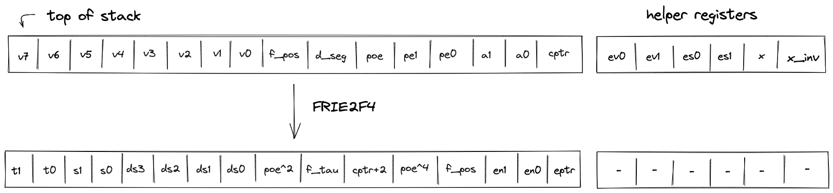
At the high-level, the operation does the following:
- Computes the domain value based on values of and .
- Using and , folds the query values into a single value .
- Compares the previously folded value to the appropriate value of to verify that the folding of the previous layer was done correctly.
- Computes the new value of as (this is done in two steps to keep the constraint degree low).
- Increments the layer address pointer by .
- Shifts the stack by to the left. This moves an element from the stack overflow table into the last position on the stack top.
To keep the degree of the constraints low, a number of intermediate values are used. Specifically, the operation relies on all helper registers, and also uses the first elements of the stack at the next state for degree reduction purposes. Thus, once the operation has been executed, the top elements of the stack can be considered to be "garbage".
TODO: add detailed constraint descriptions. See discussion here.
The effect on the rest of the stack is:
- Left shift starting from position .
HORNERBASE
The HORNERBASE operation performs steps of the Horner method for evaluating a polynomial with coefficients over the base field at a point in the quadratic extension field. More precisely, it performs the following update to the accumulator on the stack
where are the coefficients of the polynomial, the evaluation point, the current accumulator value and the updated accumulator value.
The stack for the operation is expected to be arranged as follows:
- The first stack elements contain base field elements representing the current 8-element batch of coefficients for the polynomial being evaluated.
- The next stack elements are irrelevant for the operation and unaffected by it.
- The next stack element contains the value of the memory pointer
alpha_ptrto the evaluation point . The word address containing is expected to have layout . - The next stack elements contain the value of the current accumulator .
The diagram below illustrates the stack transition for HORNERBASE operation.
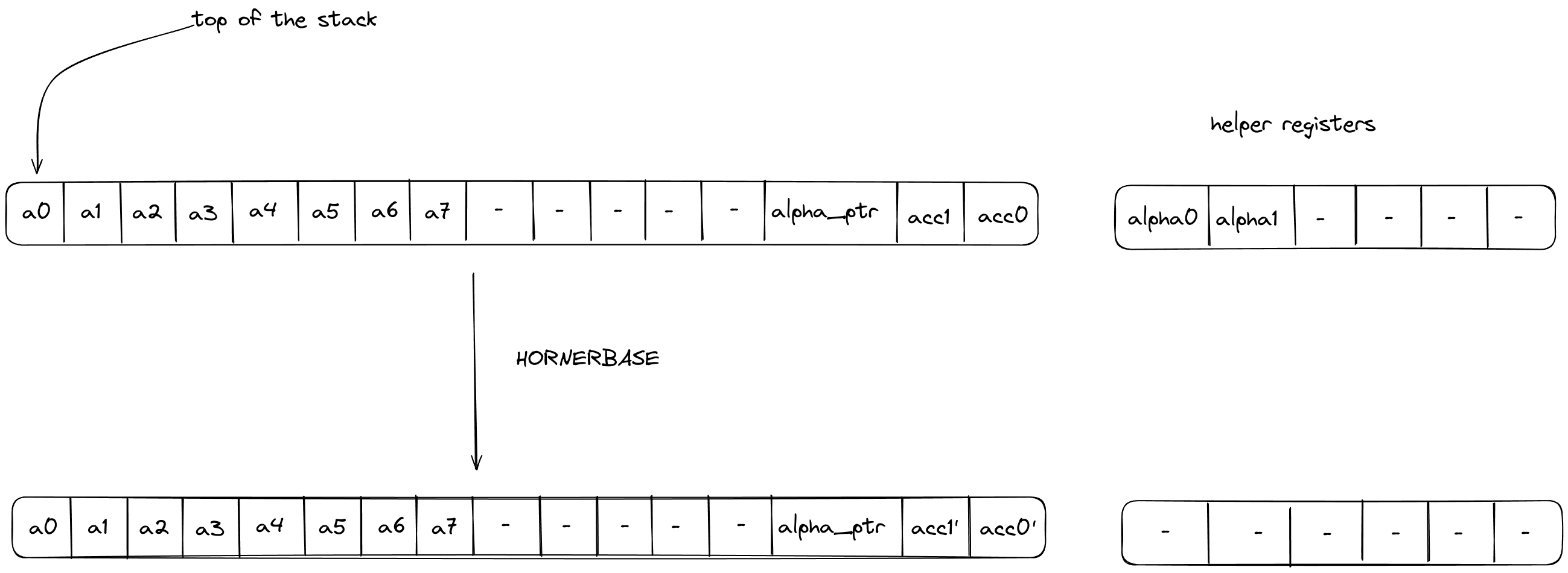
After calling the operation:
- Stack elements and will contain the value of the updated accumulator i.e., .
The effect on the rest of the stack is:
- No change.
The HORNERBASE makes one memory access request:
HORNEREXT
The HORNEREXT operation performs steps of the Horner method for evaluating a polynomial with coefficients over the quadratic extension field at a point in the quadratic extension field. More precisely, it performs the following update to the accumulator on the stack
where are the coefficients of the polynomial, the evaluation point, the current accumulator value and the updated accumulator value.
The stack for the operation is expected to be arranged as follows:
- The first stack elements contain base field elements representing the current 4-element batch of coefficients, in the quadratic extension field, for the polynomial being evaluated.
- The next stack elements are irrelevant for the operation and unaffected by it.
- The next stack element contains the value of the memory pointer
alpha_ptrto the evaluation point . The word address containing is expected to have layout . - The next stack elements contain the value of the current accumulator .
The diagram below illustrates the stack transition for HORNEREXT operation.
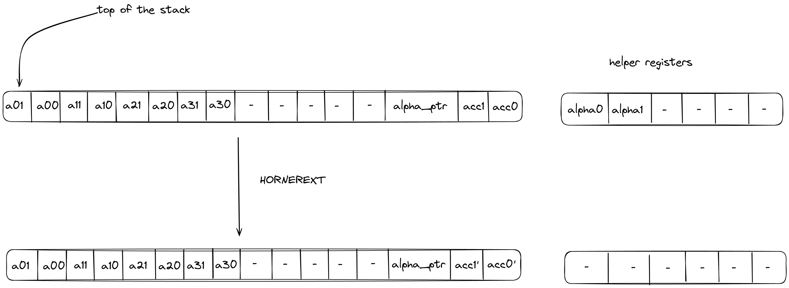
After calling the operation:
- Stack elements and will contain the value of the updated accumulator i.e., .
The effect on the rest of the stack is:
- No change.
The HORNEREXT makes one memory access request:
Range Checker
Miden VM relies very heavily on 16-bit range-checks (checking if a value of a field element is between and ). For example, most of the u32 operations need to perform between two and four 16-bit range-checks per operation. Similarly, operations involving memory (e.g. load and store) require two 16-bit range-checks per operation.
Thus, it is very important for the VM to be able to perform a large number of 16-bit range checks very efficiently. In this note we describe how this can be achieved using the LogUp lookup argument.
8-bit range checks
First, let's define a construction for the simplest possible 8-bit range-check. This can be done with a single column as illustrated below.
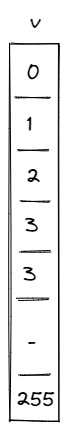
For this to work as a range-check we need to enforce a few constraints on this column:
- The value in the first row must be .
- The value in the last row must be .
- As we move from one row to the next, we can either keep the value the same or increment it by .
Denoting as the value of column in the current row, and as the value of column in the next row, we can enforce the last condition as follows:
Together, these constraints guarantee that all values in column are between and (inclusive).
We can then make use of the LogUp lookup argument by adding another column which will keep a running sum that is the logarithmic derivative of the product of values in the column. The transition constraint for would look as follows:
Since constraints cannot include divisions, the constraint would actually be expressed as the following degree 2 constraint:
Using these two columns we can check if some other column in the execution trace is a permutation of values in . Let's call this other column . We can compute the logarithmic derivative for as a running sum in the same way as we compute it for . Then, we can check that the last value in is the same as the final value for the running sum of .
While this approach works, it has a couple of limitations:
- First, column must contain all values between and . Thus, if column does not contain one of these values, we need to artificially add this value to somehow (i.e., we need to pad with extra values).
- Second, assuming is the length of execution trace, we can range-check at most values. Thus, if we wanted to range-check more than values, we'd need to introduce another column similar to .
We can get rid of both requirements by including the multiplicity of the value into the calculation of the logarithmic derivative for LogUp, which will allow us to specify exactly how many times each value needs to be range-checked.
A better construction
Let's add one more column to our table to keep track of how many times each value should be range-checked.
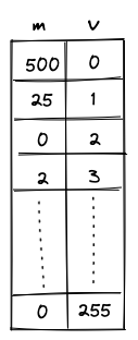
The transition constraint for is now as follows:
This addresses the limitations we had as follows:
- We no longer need to pad the column we want to range-check with extra values because we can skip the values we don't care about by setting the multiplicity to .
- We can range check as many unique values as there are rows in the trace, and there is essentially no limit to how many times each of these values can be range-checked. (The only restriction on the multiplicity value is that it must be less than the size of the set of lookup values. Therefore, for long traces where , must hold, and for short traces must be true.)
Additionally, the constraint degree has not increased versus the naive approach, and the only additional cost is a single trace column.
16-bit range checks
To support 16-bit range checks, let's try to extend the idea of the 8-bit table. Our 16-bit table would look like so (the only difference is that column now has to end with value ):
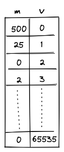
While this works, it is rather wasteful. In the worst case, we'd need to enumerate over 65K values, most of which we may not actually need. It would be nice if we could "skip over" the values that we don't want. One way to do this could be to add bridge rows between two values to be range checked and add constraints to enforce the consistency of the gap between these bridge rows.
If we allow gaps between two consecutive rows to only be 0 or powers of 2, we could enforce a constraint:
This constraint has a degree 9. This construction allows the minimum trace length to be 1024.
We could go even further and allow the gaps between two consecutive rows to only be 0 or powers of 3. In this case we would enforce the constraint:
This allows us to reduce the minimum trace length to 64.
To find out the number of bridge rows to be added in between two values to be range checked, we represent the gap between them as a linear combination of powers of 3, ie,
Then for each except the first, we add a bridge row at a gap of .
Miden approach
This construction is implemented in Miden with the following requirements, capabilities and constraints.
Requirements
- 2 columns of the main trace: , where contains the value being range-checked and is the number of times the value is checked (its multiplicity).
- 1 bus to ensure that the range checks performed in the range checker match those requested by other VM components (the stack and the memory chiplet).
Capabilities
The construction gives us the following capabilities:
- For long traces (when ), we can do an essentially unlimited number of arbitrary 16-bit range-checks.
- For short traces (), we can range-check slightly fewer than unique values, but there is essentially no practical limit to the total number of range checks.
Execution trace
The range checker's execution trace looks as follows:
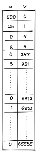
The columns have the following meanings:
- is the multiplicity column that indicates the number of times the value in that row should be range checked (included into the computation of the logarithmic derivative).
- contains the values to be range checked.
- These values go from to . Values must either stay the same or increase by powers of 3 less than or equal to .
- The final 2 rows of the 16-bit section of the trace must both equal . The extra value of is required in order to pad the trace so the bus column can be computed correctly.
Execution trace constraints
First, we need to constrain that the consecutive values in the range checker are either the same or differ by powers of 3 that are less than or equal to .
In addition to the transition constraints described above, we also need to enforce the following boundary constraints:
- The value of in the first row is .
- The value of in the last row is .
Communication bus
is the bus that connects components which require 16-bit range checks to the values in the range checker. The bus constraints are defined by the components that use it to communicate.
Requests are sent to the range checker bus by the following components:
- The Stack sends requests for 16-bit range checks during some
u32operations. - The Memory chiplet sends requests for 16-bit range checks against the values in the and trace columns to enforce internal consistency.
Responses are provided by the range checker using the transition constraint for the LogUp construction described above.
To describe the complete transition constraint for the bus, we'll define the following variables:
- : the boolean flag that indicates whether or not a stack operation requiring range checks is occurring. This flag has degree 3.
- : the boolean flag that indicates whether or not a memory operation requiring range checks is occurring. This flag has degree 3.
- : the values for which range checks are requested from the stack when is set.
- : the values for which range checks are requested from the memory chiplet when is set.
As previously mentioned, constraints cannot include divisions, so the actual constraint which is applied will be the equivalent expression in which all denominators have been multiplied through, which is degree 9.
If is initialized to and the values sent to the bus by other VM components match those that are range-checked in the trace, then at the end of the trace we should end up with .
Therefore, in addition to the transition constraint described above, we also need to enforce the following boundary constraints:
- The value of in the first row .
- The value of in the last row .
Chiplets
The Chiplets module contains specialized components dedicated to accelerating complex computations. Each chiplet specializes in executing a specific type of computation and is responsible for proving both the correctness of its computations and its own internal consistency.
Currently, Miden VM relies on 4 chiplets:
- The Hash Chiplet (also referred to as the Hasher), used to compute Rescue Prime Optimized hashes both for sequential hashing and for Merkle tree hashing.
- The Bitwise Chiplet, used to compute bitwise operations (e.g.,
AND,XOR) over 32-bit integers. - The Memory Chiplet, used to support random-access memory in the VM.
- The Kernel ROM Chiplet, used to enable executing kernel procedures during the
SYSCALLoperation.
Each chiplet executes its computations separately from the rest of the VM and proves the internal correctness of its execution trace in a unique way that is specific to the operation(s) it supports. These methods are described by each chiplet’s documentation.
Chiplets module trace
The execution trace of the Chiplets module is generated by stacking the execution traces of each of its chiplet components. Because each chiplet is expected to generate significantly fewer trace rows than the other VM components (i.e., the decoder, stack, and range checker), stacking them enables the same functionality without adding as many columns to the execution trace.
Each chiplet is identified within the Chiplets module by one or more chiplet selector columns which cause its constraints to be selectively applied.
The result is an execution trace of 17 trace columns, which allows space for the widest chiplet component (the hash chiplet) and a column to select for it.
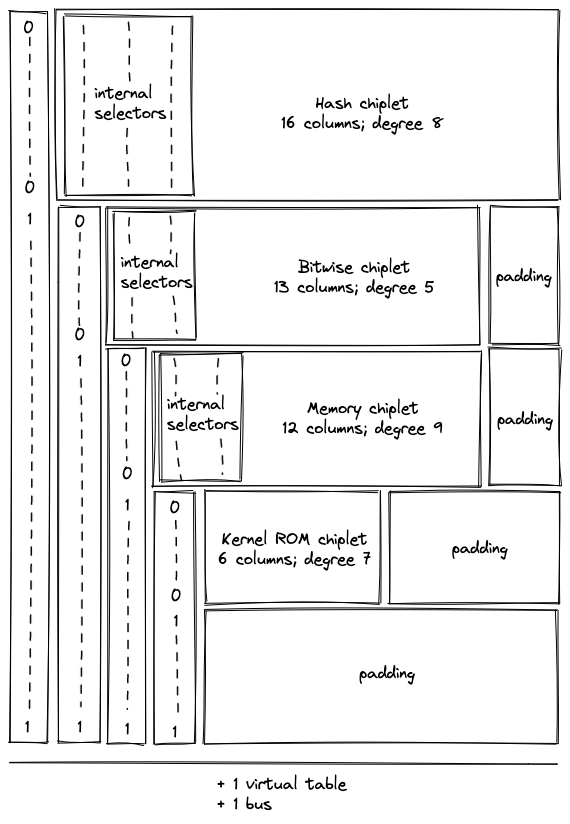
During the finalization of the overall execution trace, the chiplets' traces (including internal selectors) are appended to the trace of the Chiplets module one after another, as pictured. Thus, when one chiplet's trace ends, the trace of the next chiplet starts in the subsequent row.
Additionally, a padding segment is added to the end of the Chiplets module's trace so that the number of rows in the table always matches the overall trace length of the other VM processors, regardless of the length of the chiplet traces. The padding will simply contain zeroes.
Chiplets order
The order in which the chiplets are stacked is determined by the requirements of each chiplet, including the width of its execution trace and the degree of its constraints.
For simplicity, all of the "cyclic" chiplets which operate in multi-row cycles and require starting at particular row increments should come before any non-cyclic chiplets, and these should be ordered from longest-cycle to shortest-cycle. This avoids any additional alignment padding between chiplets.
After that, chiplets are ordered by degree of constraints so that higher-degree chiplets get lower-degree chiplet selector flags.
The resulting order is as follows:
| Chiplet | Cycle Length | Internal Degree | Chiplet Selector Degree | Total Degree | Columns | Chiplet Selector Flag |
|---|---|---|---|---|---|---|
| Hash chiplet | 8 | 8 | 1 | 9 | 17 | |
| Bitwise chiplet | 8 | 3 | 2 | 5 | 13 | |
| Memory | - | 6 | 3 | 9 | 12 | |
| Kernel ROM | - | 2 | 4 | 6 | 6 | |
| Padding | - | - | - | - | - |
Additional requirements for stacking execution traces
Stacking the chiplets introduces one new complexity. Each chiplet proves its own correctness with its own set of internal transition constraints, many of which are enforced between each row in its trace and the next row. As a result, when the chiplets are stacked, transition constraints applied to the final row of one chiplet will cause a conflict with the first row of the following chiplet.
This is true for any transition constraints which are applied at every row and selected by a Chiplet Selector Flag for the current row. (Therefore cyclic transition constraints controlled by periodic columns do not cause an issue.)
This requires the following adjustments for each chiplet.
In the hash chiplet: there is no conflict, and therefore no change, since all constraints are periodic.
In the bitwise chiplet: there is no conflict, and therefore no change, since all constraints are periodic.
In the memory chiplet: all transition constraints cause a conflict. To adjust for this, the selector flag for the memory chiplet is designed to exclude its last row. Thus, memory constraints will not be applied when transitioning from the last row of the memory chiplet to the subsequent row. This is achieved without any additional increase in the degree of constraints by using as a selector instead of as seen below.
In the kernel ROM chiplet: the transition constraints applied to the column cause a conflict. It is resolved by using a virtual flag to exclude the last row, which increases the degree of these constraints to .
Operation labels
Each operation supported by the chiplets is given a unique identifier to ensure that the requests and responses sent to the chiplets bus () are indeed processed by the intended chiplet for that operation and that chiplets which support more than one operation execute the correct one.
The labels are composed from the flag values of the chiplet selector(s) and internal operation selectors (if applicable). The unique label of the operation is computed as the binary aggregation of the combined selectors plus , note that the combined flag is represented in big-endian, so the bit representation below is reversed.
Note: We started moving away from this scheme with the memory chiplet, which more simply prepends the chiplet selector to the label (without reversing or adding 1).
| Operation | Chiplet Selector Flag | Internal Selector Flag | Combined Flag | Label |
|---|---|---|---|---|
HASHER_LINEAR_HASH | 3 | |||
HASHER_MP_VERIFY | 11 | |||
HASHER_MR_UPDATE_OLD | 7 | |||
HASHER_MR_UPDATE_NEW | 15 | |||
HASHER_RETURN_HASH | 1 | |||
HASHER_RETURN_STATE | 9 | |||
BITWISE_AND | 2 | |||
BITWISE_XOR | 6 | |||
MEMORY_WRITE_ELEMENT | 24 | |||
MEMORY_WRITE_WORD | 25 | |||
MEMORY_READ_ELEMENT | 26 | |||
MEMORY_READ_WORD | 27 | |||
KERNEL_PROC_CALL | 8 |
Chiplets module constraints
Chiplet constraints
Each chiplet's internal constraints are defined in the documentation for the individual chiplets. To ensure that constraints are only ever selected for one chiplet at a time, the module's selector columns are combined into flags. Each chiplet's internal constraints are multiplied by its chiplet selector flag, and the degree of each constraint is correspondingly increased.
This gives the following sets of constraints:
In the above:
- each represent an internal constraint from the indicated chiplet.
- indicates the degree of the specified constraint.
- flags are applied in a like manner for all internal constraints in each respective chiplet.
- the selector for the memory chiplet excludes the last row of the chiplet (as discussed above).
Chiplet selector constraints
We also need to ensure that the chiplet selector columns are set correctly. Although there are three columns for chiplet selectors, the stacked trace design means that they do not all act as selectors for the entire trace. Thus, selector constraints should only be applied to selector columns when they are acting as selectors.
- acts as a selector for the entire trace.
- acts as a selector column when .
- acts as a selector column when and .
- acts as a selector column when , , and .
Two conditions must be enforced for columns acting as chiplet selectors.
- When acting as a selector, the value in the selector column must be binary.
- When acting as a selector, the value in the selector column may only change from .
The following constraints ensure that selector values are binary.
The following constraints ensure that the chiplets are stacked correctly by restricting selector values so they can only change from .
In other words, the above constraints enforce that if a selector is in the current row, then it must be either or in the next row; if it is in the current row, it must be in the next row.
Chiplets bus
The chiplets must be explicitly connected to the rest of the VM in order for it to use their operations. This connection must prove that all specialized operations which a given VM component claimed to offload to one of the chiplets were in fact executed by the correct chiplet with the same set of inputs and outputs as those used by the offloading component.
This is achieved via a bus called where a request can be sent to any chiplet and a corresponding response will be sent back by that chiplet.
The bus is implemented as a single running product column where:
- Each request is “sent” by computing an operation-specific lookup value from an operation-specific label, the operation inputs, and the operation outputs, and then dividing it out of the running product column.
- Each chiplet response is “sent” by computing the same operation-specific lookup value from the label, inputs, and outputs, and then multiplying it into the running product column.
Thus, if the requests and responses match, then the bus column will start and end with the value . This condition is enforced by boundary constraints on the column.
Note that the order of the requests and responses does not matter, as long as they are all included in . In fact, requests and responses for the same operation will generally occur at different cycles.
Chiplets bus constraints
The chiplets bus constraints are defined by the components that use it to communicate.
Lookup requests are sent to the chiplets bus by the following components:
- The stack sends requests for bitwise, memory, and cryptographic hash operations.
- The decoder sends requests for hash operations for program block hashing.
- The decoder sends a procedure access request to the Kernel ROM chiplet for each
SYSCALLduring program block hashing.
Responses are provided by the hash, bitwise, memory, and kernel ROM chiplets.
Chiplets virtual table
Some chiplets require the use of a virtual table to maintain and enforce the correctness of their internal state. Because the length of these virtual tables does not exceed the length of the chiplets themselves, a single virtual table called can be shared by all chiplets.
Currently, the chiplets virtual table combines two virtual tables:
- the hash chiplet's sibling table
- the kernel ROM chiplet's kernel procedure table
To combine these correctly, the running product column for this table must be constrained not only at the beginning and the end of the trace, but also where the hash chiplet ends and where the kernel ROM chiplet begins. These positions can be identified using the chiplet selector columns.
Chiplets virtual table constraints
The expected boundary values for each chiplet's portion of the virtual table must be enforced. This can be done as follows.
For the sibling table to be properly constrained, the value of the running product column must be when the sibling table starts and finishes. This can be achieved by:
- enforcing a boundary constraint for at the first row
- using the following transition constraint to enforce that the value is once again at the last cycle of the hash chiplet.
For the kernel procedure table to be properly constrained, the value must be when it starts, and it must be equal to the product of all of the kernel ROM procedures when it finishes. This can be achieved by:
- enforcing a boundary constraint against the last row for the value of all of the kernel ROM procedures
- using the following transition constraint to enforce that when the active chiplet changes to the kernel ROM chiplet the value is .
Hash chiplet
Miden VM "offloads" all hash-related computations to a separate hash processor. This chiplet supports executing the Rescue Prime Optimized hash function (or rather a specific instantiation of it) in the following settings:
- A single permutation of Rescue Prime Optimized.
- A simple 2-to-1 hash.
- A linear hash of field elements.
- Merkle path verification.
- Merkle root update.
The chiplet can be thought of as having a small instruction set of instructions. These instructions are listed below, and examples of how these instructions are used by the chiplet are described in the following sections.
| Instruction | Description |
|---|---|
HR | Executes a single round of the VM's native hash function. All cycles which are not one less than a multiple of execute this instruction. That is, the chiplet executes this instruction on cycles , but not , and then again, , but not etc. |
BP | Initiates computation of a single permutation, a 2-to-1 hash, or a linear hash of many elements. This instruction can be executed only on cycles which are multiples of , and it can also be executed concurrently with an HR instruction. |
MP | Initiates Merkle path verification computation. This instruction can be executed only on cycles which are multiples of , and it can also be executed concurrently with an HR instruction. |
MV | Initiates Merkle path verification for the "old" node value during Merkle root update computation. This instruction can be executed only on cycles which are multiples of , and it can also be executed concurrently with an HR instruction. |
MU | Initiates Merkle path verification for the "new" node value during Merkle root update computation. This instruction can be executed only on cycles which are multiples of , and it can also be executed concurrently with an HR instruction. |
HOUT | Returns the result of the currently running computation. This instruction can be executed only on cycles which are one less than a multiple of (e.g. , etc.). |
SOUT | Returns the whole hasher state. This instruction can be executed only on cycles which are one less than a multiple of , and only if the computation was started using BP instruction. |
ABP | Absorbs a new set of elements into the hasher state when computing a linear hash of many elements. This instruction can be executed only on cycles which are one less than a multiple of , and only if the computation was started using BP instruction. |
MPA | Absorbs the next Merkle path node into the hasher state during Merkle path verification computation. This instruction can be executed only on cycles which are one less than a multiple of , and only if the computation was started using MP instruction. |
MVA | Absorbs the next Merkle path node into the hasher state during Merkle path verification for the "old" node value during Merkle root update computation. This instruction can be executed only on cycles which are one less than a multiple of , and only if the computation was started using MV instruction. |
MUA | Absorbs the next Merkle path node into the hasher state during Merkle path verification for the "new" node value during Merkle root update computation. This instruction can be executed only on cycles which are one less than a multiple of , and only if the computation was started using Mu instruction. |
Chiplet trace
Execution trace table of the chiplet consists of trace columns and periodic columns. The structure of the table is such that a single permutation of the hash function can be computed using table rows. The layout of the table is illustrated below.
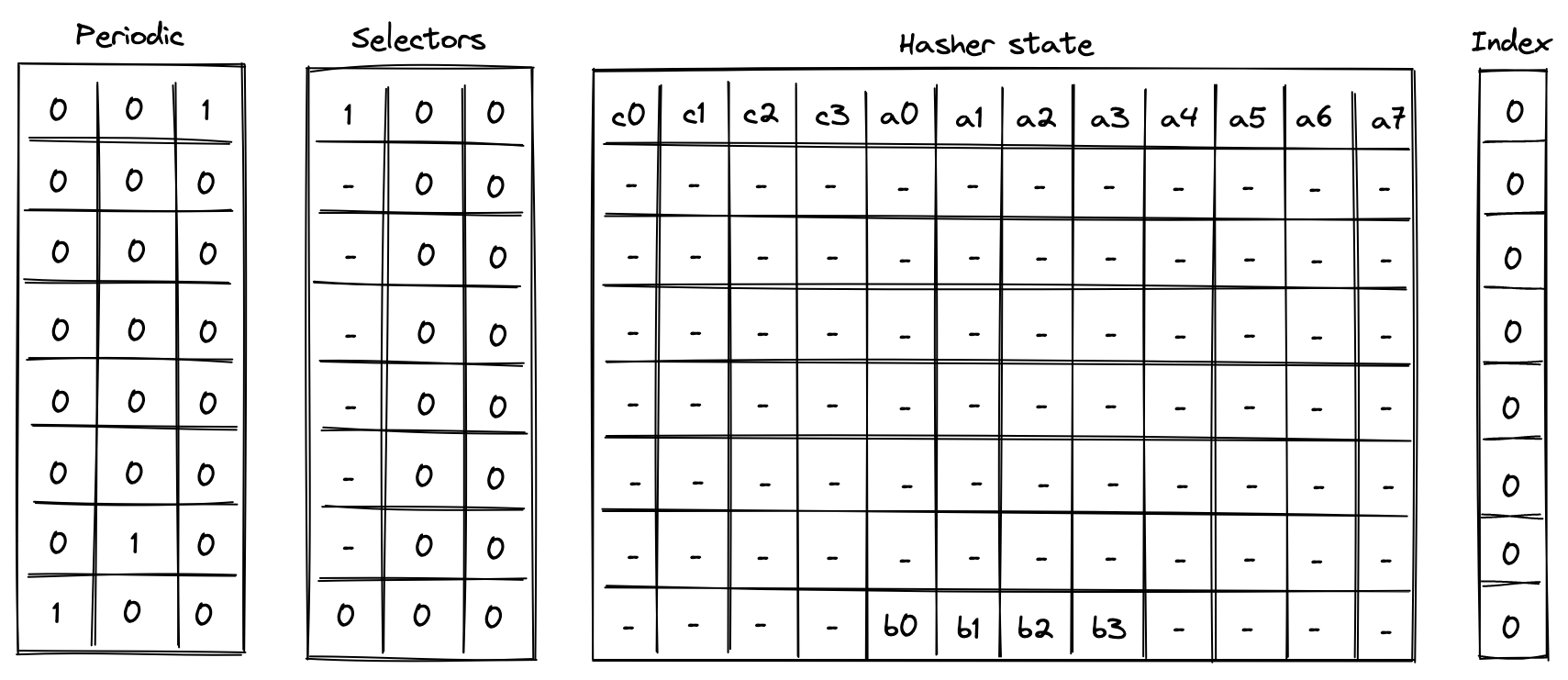
The meaning of the columns is as follows:
- Three periodic columns , , and are used to help select the instruction executed at a given row. All of these columns contain patterns which repeat every rows. For the pattern is zeros followed by one, helping us identify the last row in the cycle. For the pattern is zeros, one, and zero, which can be used to identify the second-to-last row in a cycle. For the pattern is one followed by zeros, which can identify the first row in the cycle.
- Three selector columns , , and . These columns can contain only binary values (ones or zeros), and they are also used to help select the instruction to execute at a given row.
- Twelve hasher state columns . These columns are used to hold the hasher state for each round of the hash function permutation. The state is laid out as follows:
- The first four columns () are reserved for capacity elements of the state. When the state is initialized for hash computations, should be set to if the number of elements to be hashed is a multiple of the rate width (). Otherwise, should be set to . should be set to the domain value if a domain has been provided (as in the case of control block hashing). All other capacity elements should be set to 's.
- The next eight columns () are reserved for the rate elements of the state. These are used to absorb the values to be hashed. Once the permutation is complete, hash output is located in the first four rate columns ().
- One index column . This column is used to help with Merkle path verification and Merkle root update computations.
In addition to the columns described above, the chiplet relies on two running product columns which are used to facilitate multiset checks (similar to the ones described here). These columns are:
- - which is used to tie the chiplet table with the main VM's stack and decoder. That is, values representing inputs consumed by the chiplet and outputs produced by the chiplet are multiplied into , while the main VM stack (or decoder) divides them out of . Thus, if the sets of inputs and outputs between the main VM stack and hash chiplet are the same, the value of should be equal to at the start and the end of the execution trace.
- - which is used to keep track of the sibling table used for Merkle root update computations. Specifically, when a root for the old leaf value is computed, we add an entry for all sibling nodes to the table (i.e., we multiply by the values representing these entries). When the root for the new leaf value is computed, we remove the entries for the nodes from the table (i.e., we divide by the value representing these entries). Thus, if both computations used the same set of sibling nodes (in the same order), the sibling table should be empty by the time Merkle root update procedure completes (i.e., the value of would be ).
Instruction flags
As mentioned above, chiplet instructions are encoded using a combination of periodic and selector columns. These columns can be used to compute a binary flag for each instruction. Thus, when a flag for a given instruction is set to , the chiplet executes this instruction. Formulas for computing instruction flags are listed below.
| Flag | Value | Notes |
|---|---|---|
| Set to on the first steps of every -step cycle. | ||
| Set to when selector flags are on rows which are multiples of . | ||
| Set to when selector flags are on rows which are multiples of . | ||
| Set to when selector flags are on rows which are multiples of . | ||
| Set to when selector flags are on rows which are multiples of . | ||
| Set to when selector flags are on rows which are less than a multiple of . | ||
| Set to when selector flags are on rows which are less than a multiple of . | ||
| Set to when selector flags are on rows which are less than a multiple of . | ||
| Set to when selector flags are on rows which are less than a multiple of . | ||
| Set to when selector flags are on rows which are less than a multiple of . | ||
| Set to when selector flags are on rows which are less than a multiple of . |
A few additional notes about flag values:
- With the exception of , all flags are mutually exclusive. That is, if one flag is set to , all other flats are set to .
- With the exception of , computing flag values involves multiplications, and thus the degree of these flags is .
- We can also define a flag . This flag will be set to when either or in the current row.
- We can define a flag . This flag will be set to when either or in the next row.
We also impose the following restrictions on how values in selector columns can be updated:
- Values in columns and must be copied over from one row to the next, unless or indicating the
houtorsoutflag is set for the current or the next row. - Value in must be set to if for the previous row, and to if any of the flags , , , or are set to for the previous row.
The above rules ensure that we must finish one computation before starting another, and we can't change the type of the computation before the computation is finished.
Computation examples
Single permutation
Computing a single permutation of Rescue Prime Optimized hash function involves the following steps:
- Initialize hasher state with field elements.
- Apply Rescue Prime Optimized permutation.
- Return the entire hasher state as output.
The chiplet accomplishes the above by executing the following instructions:
[BP, HR]                 // init state and execute a hash round (concurrently)
HR HR HR HR HR HR        // execute 6 more hash rounds
SOUT                     // return the entire state as output
Execution trace for this computation would look as illustrated below.
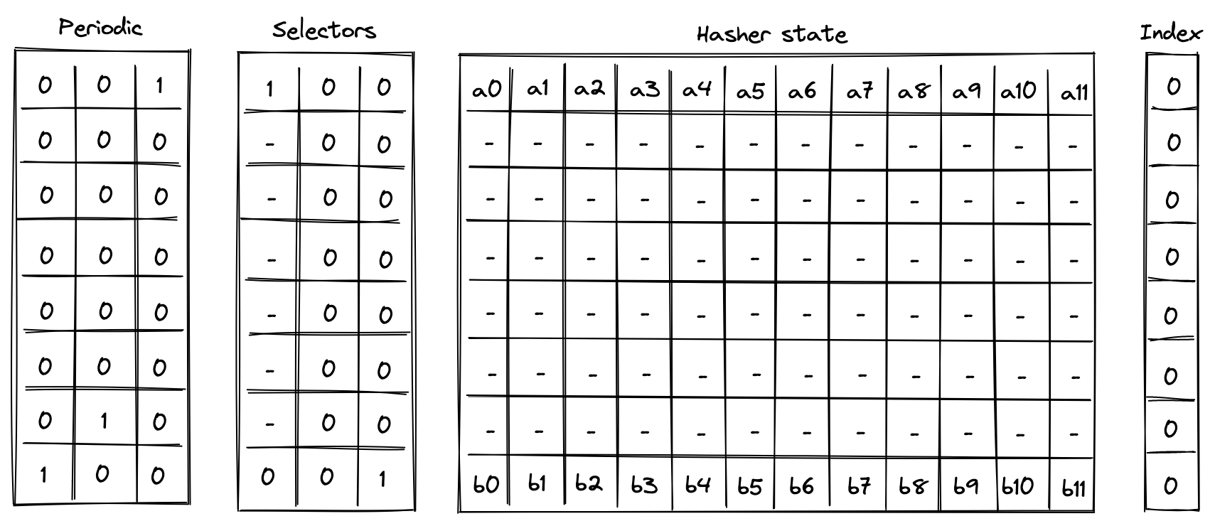
In the above is the input state of the hasher, and is the output state of the hasher.
Simple 2-to-1 hash
Computing a 2-to-1 hash involves the following steps:
- Initialize hasher state with field elements, setting the second capacity element to if the domain is provided (as in the case of control block hashing) or else , and the remaining capacity elements to .
- Apply Rescue Prime Optimized permutation.
- Return elements of the hasher state as output.
The chiplet accomplishes the above by executing the following instructions:
[BP, HR]                 // init state and execute a hash round (concurrently)
HR HR HR HR HR HR        // execute 6 more hash rounds
HOUT                     // return elements 4, 5, 6, 7 of the state as output
Execution trace for this computation would look as illustrated below.
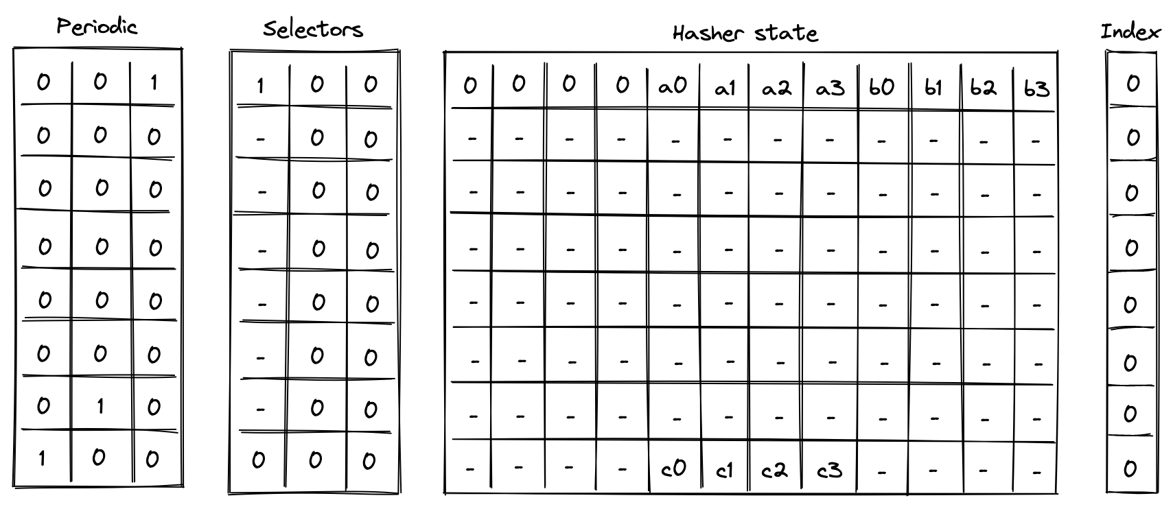
In the above, we compute the following:
Linear hash of n elements
Computing a linear hash of elements consists of the following steps:
- Initialize hasher state with the first elements, setting the first capacity register to if is a multiple of the rate width () or else , and the remaining capacity elements to .
- Apply Rescue Prime Optimized permutation.
- Absorb the next set of elements into the state (up to elements), while keeping capacity elements unchanged.
- Repeat steps 2 and 3 until all elements have been absorbed.
- Return elements of the hasher state as output.
The chiplet accomplishes the above by executing the following instructions (for hashing elements):
[BP, HR]                    // init state and execute a hash round (concurrently)
HR HR HR HR HR HR           // execute 6 more hash rounds
ABP                         // absorb the next set of elements into the state
HR HR HR HR HR HR HR        // execute 7 hash rounds
HOUT                        // return elements 4, 5, 6, 7 of the state as output
Execution trace for this computation would look as illustrated below.
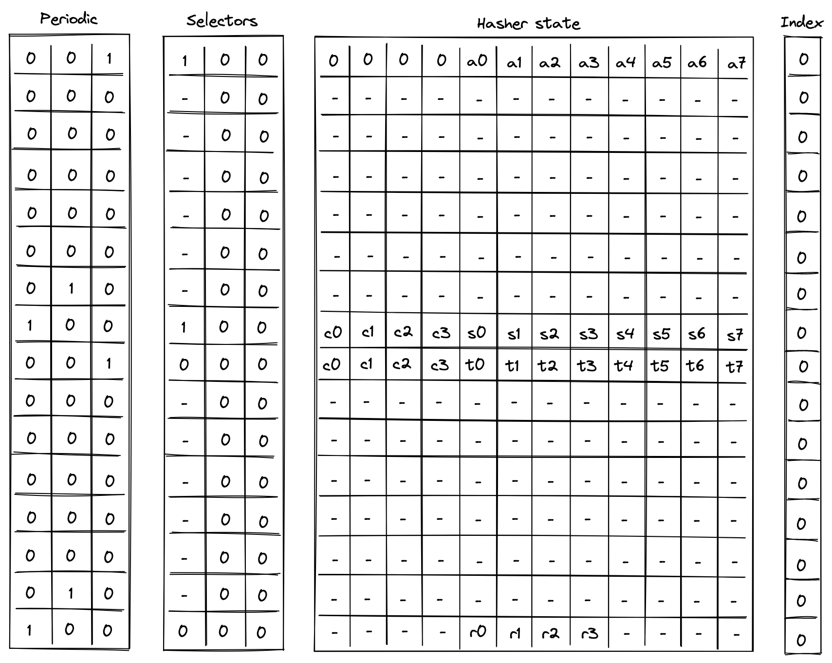
In the above, the value absorbed into hasher state between rows and is the delta between values and . Thus, if we define for , the above computes the following:
Verify Merkle path
Verifying a Merkle path involves the following steps:
- Initialize hasher state with the leaf and the first node of the path, setting all capacity elements to s. a. Also, initialize the index register to the leaf's index value.
- Apply Rescue Prime Optimized permutation. a. Make sure the index value doesn't change during this step.
- Copy the result of the hash to the next row, and absorb the next node of the Merkle path into the hasher state. a. Remove a single bit from the index, and use it to determine how to place the copied result and absorbed node in the state.
- Repeat steps 2 and 3 until all nodes of the Merkle path have been absorbed.
- Return elements of the hasher state as output. a. Also, make sure the index value has been reduced to .
The chiplet accomplishes the above by executing the following instructions (for Merkle tree of depth ):
[MP, HR]                    // init state and execute a hash round (concurrently)
HR HR HR HR HR HR           // execute 6 more hash rounds
MPA                         // copy result & absorb the next node into the state
HR HR HR HR HR HR HR        // execute 7 hash rounds
HOUT                        // return elements 4, 5, 6, 7 of the state as output
Suppose we have a Merkle tree as illustrated below. This Merkle tree has leaves, each of which consists of field elements. For example, leaf consists of elements , leaf be consists of elements etc.
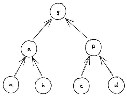
If we wanted to verify that leaf is in fact in the tree, we'd need to compute the following hashes:
And if , we can be convinced that is in fact in the tree at position . Execution trace for this computation would look as illustrated below.
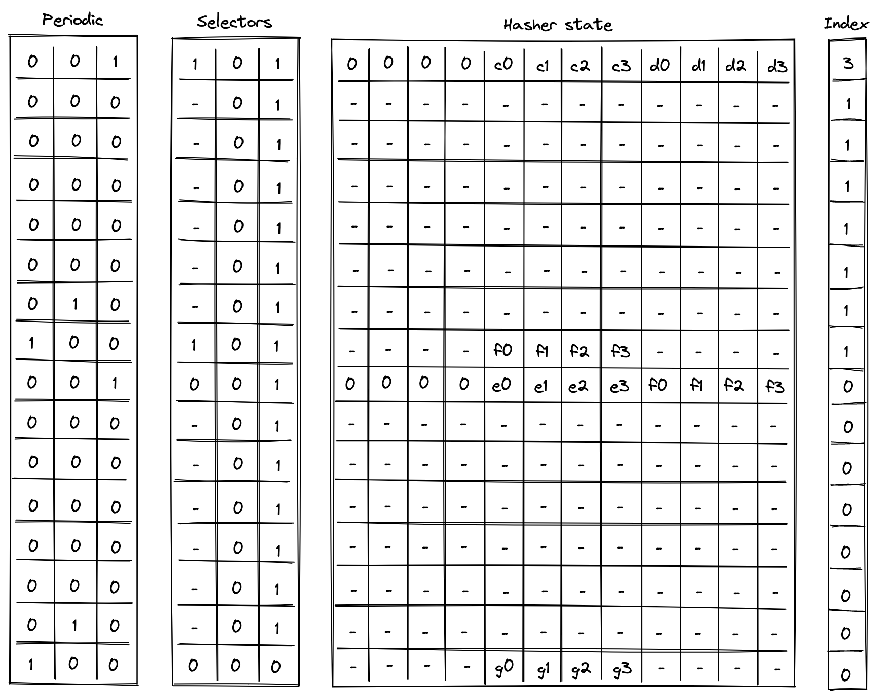
In the above, the prover provides values for nodes and non-deterministically.
Update Merkle root
Updating a node in a Merkle tree (which also updates the root of the tree) can be simulated by verifying two Merkle paths: the path that starts with the old leaf and the path that starts with the new leaf.
Suppose we have the same Merkle tree as in the previous example, and we want to replace node with node . The computations we'd need to perform are:
Then, as long as , and the same values were used for and in both computations, we can be convinced that the new root of the tree is .
The chiplet accomplishes the above by executing the following instructions:
// verify the old merkle path
[MV, HR]                    // init state and execute a hash round (concurrently)
HR HR HR HR HR HR           // execute 6 more hash rounds
MPV                         // copy result & absorb the next node into the state
HR HR HR HR HR HR HR        // execute 7 hash rounds
HOUT                        // return elements 4, 5, 6, 7 of the state as output

// verify the new merkle path
[MU, HR]                    // init state and execute a hash round (concurrently)
HR HR HR HR HR HR           // execute 6 more hash rounds
MPU                         // copy result & absorb the next node into the state
HR HR HR HR HR HR HR        // execute 7 hash rounds
HOUT                        // return elements 4, 5, 6, 7 of the state as output
The semantics of MV and MU instructions are similar to the semantics of MP instruction from the previous example (and MVA and MUA are similar to MPA) with one important difference: MV* instructions add the absorbed node (together with its index in the tree) to permutation column , while MU* instructions remove the absorbed node (together with its index in the tree) from . Thus, if the same nodes were used during both Merkle path verification, the state of should not change. This mechanism is used to ensure that the same internal nodes were used in both computations.
AIR constraints
When describing AIR constraints, we adopt the following notation: for column , we denote the value in the current row simply as , and the value in the next row of the column as . Thus, all transition constraints described in this note work with two consecutive rows of the execution trace.
Selector columns constraints
For selector columns, first we must ensure that only binary values are allowed in these columns. This can be done with the following constraints:
Next, we need to make sure that unless or , the values in columns and are copied over to the next row. This can be done with the following constraints:
Next, we need to enforce that if any of flags is set to , the next value of is . In all other cases, should be unconstrained. These flags will only be set for rows that are 1 less than a multiple of 8 (the last row of each cycle). This can be done with the following constraint:
Lastly, we need to make sure that no invalid combinations of flags are allowed. This can be done with the following constraints:
The above constraints enforce that on every step which is one less than a multiple of , if , then must also be set to . Basically, if we set , then we must make sure that either or .
Node index constraints
Node index column is relevant only for Merkle path verification and Merkle root update computations, but to simplify the overall constraint system, the same constraints will be imposed on this column for all computations.
Overall, we want values in the index column to behave as follows:
- When we start a new computation, we should be able to set to an arbitrary value.
- When a computation is finished, value in must be .
- When we absorb a new node into the hasher state we must shift the value in by one bit to the right.
- In all other cases value in should not change.
A shift by one bit to the right can be described with the following equation: , where is the value of the bit which is discarded. Thus, as long as is a binary value, the shift to the right is performed correctly, and this can be enforced with the following constraint:
Since we want to enforce this constraint only when a new node is absorbed into the hasher state, we'll define a flag for when this should happen as follows:
And then the full constraint would looks as follows:
Next, to make sure when a computation is finished , we can use the following constraint:
Finally, to make sure that the value in is copied over to the next row unless we are absorbing a new row or the computation is finished, we impose the following constraint:
To satisfy these constraints for computations not related to Merkle paths (i.e., 2-to-1 hash and liner hash of elements), we can set at the start of the computation. This guarantees that will remain until the end of the computation.
Hasher state constraints
Hasher state columns should behave as follows:
- For the first row of every -row cycle (i.e., when ), we need to apply Rescue Prime Optimized round constraints to the hasher state. For brevity, we omit these constraints from this note.
- On the th row of every -row cycle, we apply the constraints based on which transition flag is set as described in the table below.
Specifically, when absorbing the next set of elements into the state during linear hash computation (i.e., ), the first elements (the capacity portion) are carried over to the next row. For this can be described as follows:
When absorbing the next node during Merkle path computation (i.e., ), the result of the previous hash () are copied over either to or to depending on the value of , which is defined in the same way as in the previous section. For this can be described as follows:
Note, that when a computation is completed (i.e., ), the next hasher state is unconstrained.
Multiset check constraints
In this sections we describe constraints which enforce updates for multiset check columns and . These columns can be updated only on rows which are multiples of or less than a multiple of . On all other rows the values in the columns remain the same.
To simplify description of the constraints, we define the following variables. Below, we denote random values sent by the verifier after the prover commits to the main execution trace as , , etc.
In the above:
- is a transition label, composed of the operation label and the periodic columns that uniquely identify each transition function. The values in the and periodic columns are included to identify the row in the hash cycle where the operation occurs. They serve to differentiate between operations that share selectors but occur at different rows in the cycle, such as
BP, which uses at the first row in the cycle to initiate a linear hash, andABP, which uses at the last row in the cycle to absorb new elements. - is a common header which is a combination of the transition label, a unique row address, and the node index. For the unique row address, the
clkcolumn from the system component is used, but we add , because the system'sclkcolumn starts at . - , , are the first, second, and third words (4 elements) of the hasher state.
- is the third word of the hasher state but computed using the same values as used for the second word. This is needed for computing the value of below to ensure that the same values are used for the leaf node regardless of which part of the state the node comes from.
Chiplets bus constraints
As described previously, the chiplets bus , implemented as a running product column, is used to tie the hash chiplet with the main VM's stack and decoder. When receiving inputs from or returning results to the stack (or decoder), the hash chiplet multiplies by their respective values. On the other side, when sending inputs to the hash chiplet or receiving results from the chiplet, the stack (or decoder) divides by their values.
In the section below we describe only the hash chiplet side of the constraints (i.e., multiplying by relevant values). We define the values which are to be multiplied into for each operation as follows:
When starting a new simple or linear hash computation (i.e., ) or when returning the entire state of the hasher (), the entire hasher state is included into :
When starting a Merkle path computation (i.e., ), we include the leaf of the path into . The leaf is selected from the state based on value of (defined as in the previous section):
When absorbing a new set of elements into the state while computing a linear hash (i.e., ), we include deltas between the last elements of the hasher state (the rate) into :
When a computation is complete (i.e., ), we include the second word of the hasher state (the result) into :
Using the above values, we can describe the constraints for updating column as follows.
The above constraint reduces to the following under various flag conditions:
| Condition | Applied constraint |
|---|---|
| Otherwise |
Note that the degree of the above constraint is .
Sibling table constraints
Note: Although this table is described independently, it is implemented as part of the chiplets virtual table, which combines all virtual tables required by any of the chiplets into a single master table.
As mentioned previously, the sibling table (represented by running column ) is used to keep track of sibling nodes used during Merkle root update computations. For this computation, we need to enforce the following rules:
- When computing the old Merkle root, whenever a new sibling node is absorbed into the hasher state (i.e., ), an entry for this sibling should be included into .
- When computing the new Merkle root, whenever a new sibling node is absorbed into the hasher state (i.e., ), the entry for this sibling should be removed from .
To simplify the description of the constraints, we use variables and defined above and define the value representing an entry in the sibling table as follows:
Using the above value, we can define the constraint for updating as follows:
The above constraint reduces to the following under various flag conditions:
| Condition | Applied constraint |
|---|---|
| Otherwise |
Note that the degree of the above constraint is .
To make sure computation of the old Merkle root is immediately followed by the computation of the new Merkle root, we impose the following constraint:
The above means that whenever we start a new computation which is not the computation of the new Merkle root, the sibling table must be empty. Thus, after the hash chiplet computes the old Merkle root, the only way to clear the table is to compute the new Merkle root.
Together with boundary constraints enforcing that at the first and last rows of the running product column which implements the sibling table, the above constraints ensure that if a node was included into as a part of computing the old Merkle root, the same node must be removed from as a part of computing the new Merkle root. These two boundary constraints are described as part of the chiplets virtual table constraints.
Bitwise chiplet
In this note we describe how to compute bitwise AND and XOR operations on 32-bit values and the constraints required for proving correct execution.
Assume that and are field elements in a 64-bit prime field. Assume also that and are known to contain values smaller than . We want to compute , where is either bitwise AND or XOR, and is a field element containing the result of the corresponding bitwise operation.
First, observe that we can compute AND and XOR relations for single bit values as follows:
To compute bitwise operations for multi-bit values, we will decompose the values into individual bits, apply the operations to single bits, and then aggregate the bitwise results into the final result.
To perform this operation we will use a table with 12 columns, and computing a single AND or XOR operation will require 8 table rows. We will also rely on two periodic columns as shown below.
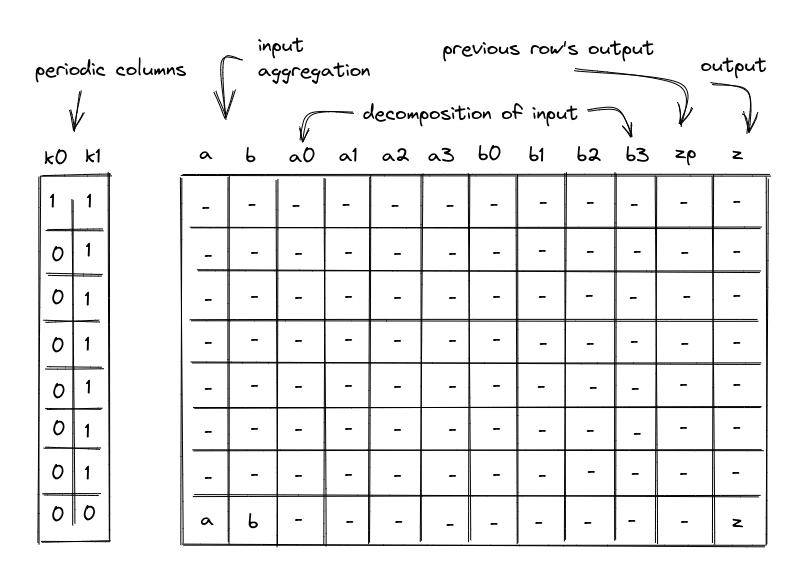
In the above, the columns have the following meanings:
- Periodic columns and . These columns contain values needed to switch various constraints on or off. contains a single one, followed by a repeating sequence of seven zeros. contains a repeating sequence of seven ones, followed by a single zero.
- Input columns and . On the first row of each 8-row cycle, the prover will set values in these columns to the upper 4 bits of the values to which a bitwise operation is to be applied. For all subsequent rows, we will append the next-most-significant 4-bit limb to each value. Thus, by the final row columns and will contain the full input values for the bitwise operation.
- Columns , , , , , , , will contain lower 4 bits of their corresponding values.
- Output column . This column represents the value of column for the prior row. For the first row, it is set to .
- Output column . This column will be used to aggregate the results of bitwise operations performed over columns , , , , , , , . By the time we get to the last row in each 8-row cycle, this column will contain the final result.
Example
Let's illustrate the above table on a concrete example. For simplicity, we'll use 16-bit values, and thus, we'll only need 4 rows to complete the operation (rather than 8 for 32-bit values). Let's say (b1010_0011_0111_1011) and (b1001_1101_1110_1010), then (b1000_0001_0110_1010). The table for this computation looks like so:
| a | b | a0 | a1 | a2 | a3 | b0 | b1 | b2 | b3 | zp | z |
|---|---|---|---|---|---|---|---|---|---|---|---|
| 10 | 9 | 0 | 1 | 0 | 1 | 1 | 0 | 0 | 1 | 0 | 8 |
| 163 | 157 | 1 | 1 | 0 | 0 | 1 | 0 | 1 | 1 | 8 | 129 |
| 2615 | 2526 | 1 | 1 | 1 | 0 | 0 | 1 | 1 | 1 | 129 | 2070 |
| 41851 | 40426 | 1 | 1 | 0 | 1 | 0 | 1 | 0 | 1 | 2070 | 33130 |
Here, in the first row, we set each of the and columns to the value of their most-significant 4-bit limb. The bit columns ( and ) in the first row contain the lower 4 bits of their corresponding values (b1010 and b1001). Column contains the result of bitwise AND for the upper 4 bits (b1000), while column contains that result for the prior row.
With every subsequent row, we inject the next-most-significant 4 bits of each value into the bit columns, increase the and columns accordingly, and aggregate the result of bitwise AND into the column, adding it to times the value of in the previous row. We set column to be the value of in the prior row. By the time we get to the last row, the column contains the result of the bitwise AND, while columns and contain their original values.
Constraints
AIR constraints needed to ensure the correctness of the above table are described below. We also add one more column to the execution trace, to allow us to select between two bitwise operations (U32AND and U32XOR).
Selectors
The Bitwise chiplet supports two operations with the following operation selectors:
U32AND:U32XOR:
The constraints must require that the selectors be binary and stay the same throughout the cycle:
Input decomposition
We need to make sure that inputs and are decomposed correctly into their individual bits. To do this, first, we need to make sure that columns , , , , , , , , can contain only binary values ( or ). This can be accomplished with the following constraints (for ranging between and ):
Then, we need to make sure that on the first row of every 8-row cycle, the values in the columns and are exactly equal to the aggregation of binary values contained in the individual bit columns , and . This can be enforced with the following constraints:
The above constraints enforce that when , and .
Lastly, we need to make sure that for all rows in an 8-row cycle except for the last one, the values in and columns are increased by the values contained in the individual bit columns and . Denoting as the value of column in the current row, and as the value of column in the next row, we can enforce these conditions as follows:
The above constraints enforce that when , and .
Output aggregation
To ensure correct aggregation of operations over individual bits, first we need to ensure that in the first row, the aggregated output value of the previous row should be 0.
Next, we need to ensure that for each row except the last, the aggregated output value must equal the previous aggregated output value in the next row.
Lastly, we need to ensure that for all rows the value in the column is computed by multiplying the previous output value (from the column in the current row) by 16 and then adding it to the bitwise operation applied to the row's set of bits of and . The entire constraint must also be multiplied by the operation selector flag to ensure it is only applied for the appropriate operation.
For U32AND, this is enforced with the following constraint:
For U32XOR, this is enforced with the following constraint:
Chiplets bus constraints
To simplify the notation for describing bitwise constraints on the chiplets bus, we'll first define variable , which represents how , , and in the execution trace are reduced to a single value. Denoting the random values received from the verifier as , etc., this can be achieved as follows.
Where, is the unique operation label of the bitwise operation.
The request side of the constraint for the bitwise operation is described in the stack bitwise operation section.
To provide the results of bitwise operations to the chiplets bus, we want to include values of , and at the last row of the cycle.
First, we'll define another intermediate variable . It will include into the product when . ( represents the value of for row of the trace.)
Then, setting , we can compute the permutation product from the bitwise chiplet as follows:
The above ensures that when (which is true for all rows in the 8-row cycle except for the last one), the product does not change. Otherwise, gets included into the product.
The response side of the bus communication can be enforced with the following constraint:
Memory chiplet
Miden VM supports linear read-write random access memory. This memory is element-addressable, meaning that a single value is located at each address, although reading and writing values to/from memory in batches of four is supported. Each value is a field element in a -bit prime field with modulus . A memory address is a field element in the range .
In this note we describe the rationale for selecting the above design and describe AIR constraints needed to support it.
The design makes extensive use of -bit range checks. An efficient way of implementing such range checks is described here.
Alternative designs
The simplest (and most efficient) alternative to the above design is contiguous write-once memory. To support such memory, we need to allocate just two trace columns as illustrated below.
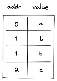
In the above, addr column holds memory address, and value column holds the field element representing the value stored at this address. Notice that some rows in this table are duplicated. This is because we need one row per memory access (either read or write operation). In the example above, value was first stored at memory address , and then read from this address.
The AIR constraints for this design are very simple. First, we need to ensure that values in the addr column either remain the same or are incremented by as we move from one row to the next. This can be achieved with the following constraint:
where is the value in addr column in the current row, and is the value in this column in the next row.
Second, we need to make sure that if the value in the addr column didn't change, the value in the value column also remained the same (i.e., a value stored in a given address can only be set once). This can be achieved with the following constraint:
where is the value in value column at the current row, and is the value in this column in the next row.
As mentioned above, this approach is very efficient: each memory access requires just trace cells.
Read-write memory
Write-once memory is tricky to work with, and many developers may need to climb a steep learning curve before they become comfortable working in this model. Thus, ideally, we'd want to support read-write memory. To do this, we need to introduce additional columns as illustrated below.
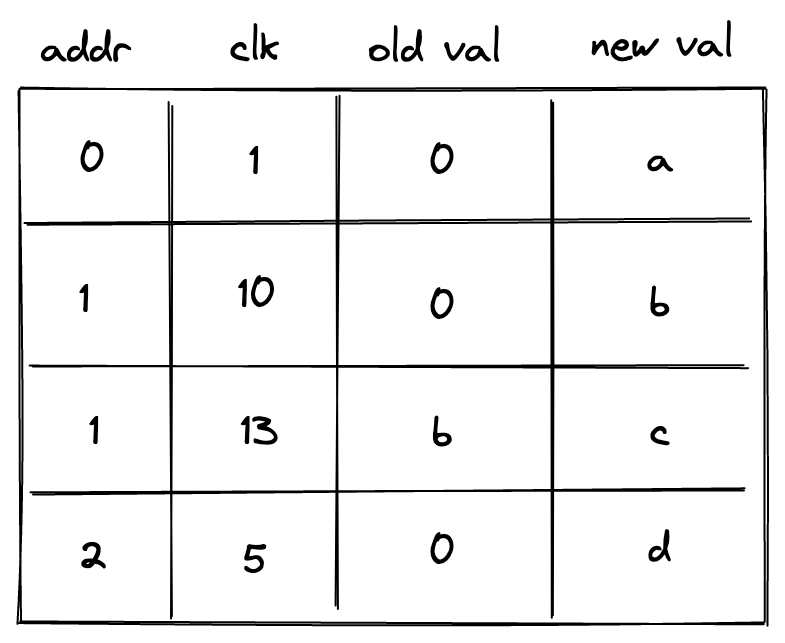
In the above, we added clk column, which keeps track of the clock cycle at which memory access happened. We also need to differentiate between memory reads and writes. To do this, we now use two columns to keep track of the value: old val contains the value stored at the address before the operation, and new val contains the value after the operation. Thus, if old val and new val are the same, it was a read operation. If they are different, it was a write operation.
The AIR constraints needed to support the above structure are as follows.
We still need to make sure memory addresses are contiguous:
Whenever memory address changes, we want to make sure that old val is set to (i.e., our memory is always initialized to ). This can be done with the following constraint:
On the other hand, if memory address doesn't change, we want to make sure that new val in the current row is the same as old val in the next row. This can be done with the following constraint:
Lastly, we need to make sure that for the same address values in clk column are always increasing. One way to do this is to perform a -bit range check on the value of , where is the reference to clk column. However, this would mean that memory operations involving the same address must happen within VM cycles from each other. This limitation would be difficult to enforce statically. To remove this limitation, we need to add two more columns as shown below:
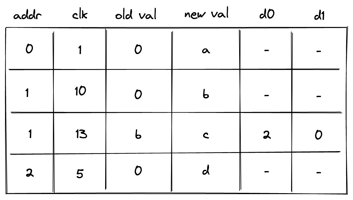
In the above column d0 contains the lower bits of while d1 contains the upper bits. The constraint needed to enforces this is as follows:
Additionally, we need to apply -bit range checks to columns d0 and d1.
Overall, the cost of reading or writing a single element is now trace cells and -bit range-checks.
Non-contiguous memory
Requiring that memory addresses are contiguous may also be a difficult limitation to impose statically. To remove this limitation, we need to introduce one more column as shown below:
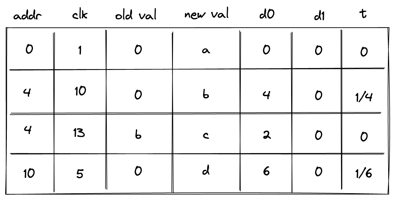
In the above, the prover sets the value in the new column t to when the address doesn't change, and to otherwise. To simplify constraint description, we'll define variable computed as follows:
Then, to make sure the prover sets the value of correctly, we'll impose the following constraints:
The above constraints ensure that whenever the address changes, and otherwise. We can then define the following constraints to make sure values in columns d0 and d1 contain either the delta between addresses or between clock cycles.
| Condition | Constraint | Comments |
|---|---|---|
When the address changes, columns d0 and d1 at the next row should contain the delta between the old and the new address. | ||
When the address remains the same, columns d0 and d1 at the next row should contain the delta between the old and the new clock cycle. |
We can combine the above constraints as follows:
The above constraint, in combination with -bit range checks against columns d0 and d1 ensure that values in addr and clk columns always increase monotonically, and also that column addr may contain duplicates, while values in clk column must be unique for a given address.
Context separation
In many situations it may be desirable to assign memories to different contexts. For example, when making a cross-contract calls, the memories of the caller and the callee should be separate. That is, the caller should not be able to access the memory of the callee and vice-versa.
To accommodate this feature, we need to add one more column as illustrated below.
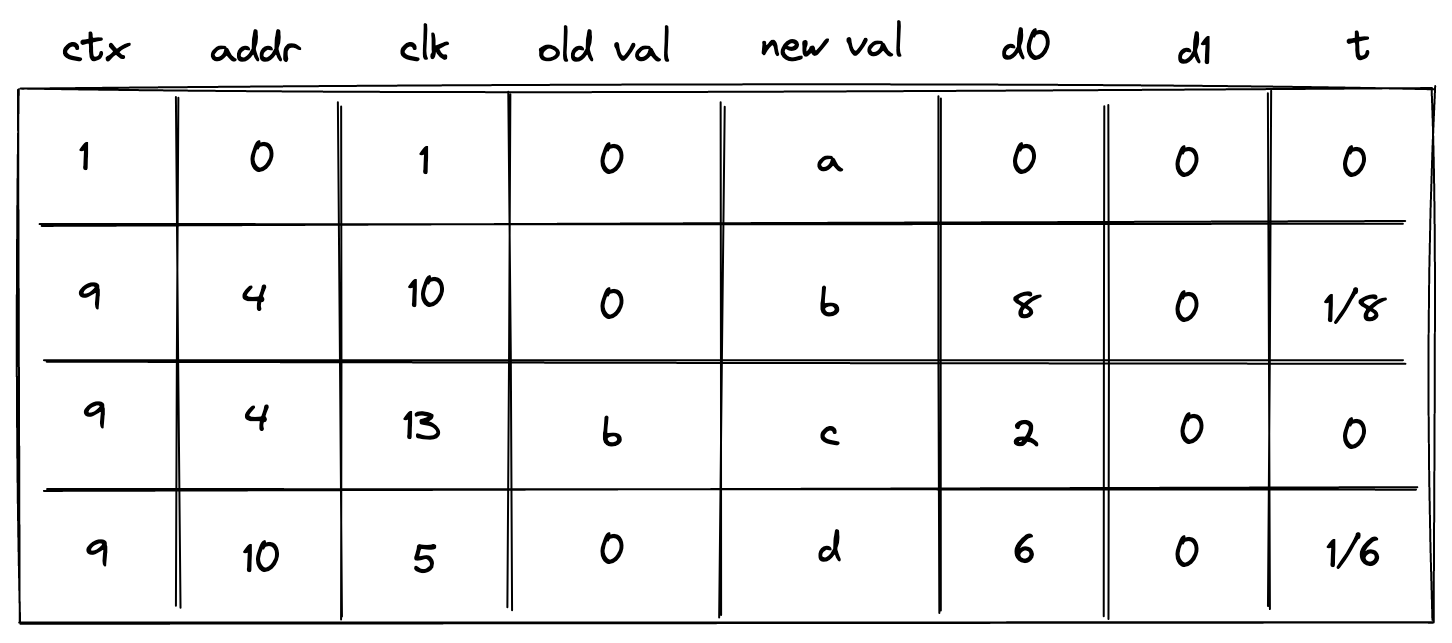
This new column ctx should behave similarly to the address column: values in it should increase monotonically, and there could be breaks between them. We also need to change how the prover populates column t:
- If the context changes,
tshould be set to the inverse , where is a reference to columnctx. - If the context remains the same but the address changes, column
tshould be set to the inverse of . - Otherwise, column
tshould be set to .
To simplify the description of constraints, we'll define two variables and as follows:
Thus, when the context changes, and otherwise. Also, when context remains the same and address changes, and otherwise.
To make sure the prover sets the value of column t correctly, we'll need to impose the following constraints:
We can then define the following constraints to make sure values in columns d0 and d1 contain the delta between contexts, between addresses, or between clock cycles.
| Condition | Constraint | Comments |
|---|---|---|
When the context changes, columns d0 and d1 at the next row should contain the delta between the old and the new contexts. | ||
| | When the context remains the same but the address changes, columns d0 and d1 at the next row should contain the delta between the old and the new addresses. | |
| | When both the context and the address remain the same, columns d0 and d1 at the next row should contain the delta between the old and the new clock cycle. |
We can combine the above constraints as follows:
The above constraint, in combination with -bit range checks against columns d0 and d1 ensure that values in ctx, addr, and clk columns always increase monotonically, and also that columns ctx and addr may contain duplicates, while the values in column clk must be unique for a given combination of ctx and addr.
Notice that the above constraint has degree .
Miden approach
While the approach described above works, it comes at significant cost. Reading or writing a single value requires trace cells and -bit range checks. Assuming a single range check requires roughly trace cells, the total number of trace cells needed grows to . This is about x worse the simple contiguous write-once memory described earlier.
Miden VM frequently needs to deal with batches of field elements, which we call words. For example, the output of Rescue Prime Optimized hash function is a single word. A single 256-bit integer value can be stored as two words (where each element contains one -bit value). Thus, we can optimize for this common use case by making the chiplet handle words as opposed to individual elements. That is, memory is still element-addressable in that each memory address stores a single field element, and memory addresses may be read or written individually. However, the chiplet also handles reading and writing elements in batches of four simultaneously, with the restriction that such batches be word-aligned addresses (i.e. the address is a multiple of 4).
The layout of Miden VM memory table is shown below:
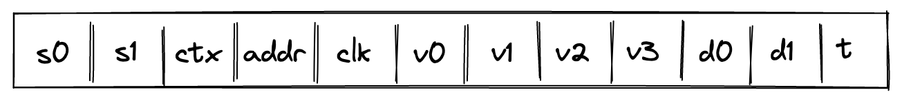
where:
rwis a selector column which is set to for read operations and for write operations.ewis a selector column which is set to when a word is being accessed, and when an element is being accessed.ctxcontains context ID. Values in this column must increase monotonically but there can be gaps between two consecutive values of up to . Also, two consecutive values can be the same.word_addrcontains the memory address of the first element in the word. Values in this column must increase monotonically for a given context but there can be gaps between two consecutive values of up to . Values in this column must be divisible by 4. Also, two consecutive values can be the same.idx0andidx1are selector columns used to identify which element in the word is being accessed. Specifically, the index within the word is computed asidx1 * 2 + idx0.- However, when
ewis set to (indicating that a word is accessed), these columns are meaningless and are set to .
- However, when
clkcontains clock cycle at which the memory operation happened. Values in this column must increase monotonically for a given context and memory word but there can be gaps between two consecutive values of up to .- Unlike the previously described approaches, we allow
clkto be constant in the same context/word address, with the restriction that when this is the case, then only reads are allowed.
- Unlike the previously described approaches, we allow
v0, v1, v2, v3columns contain field elements stored at a given context/word/clock cycle after the memory operation.- Columns
d0andd1contain lower and upper bits of the delta between two consecutive context IDs, addresses, or clock cycles. Specifically:- When the context changes within a frame, these columns contain in the "next" row.
- When the context remains the same but the word address changes within a frame, these columns contain in the "next" row.
- When both the context and the word address remain the same within a frame, these columns contain in the "next" row.
- Column
tcontains the inverse of the delta between two consecutive context IDs, addresses, or clock cycles. Specifically:- When the context changes within a frame, this column contains the inverse of in the "next" row.
- When the context remains the same but the word address changes within a frame, this column contains the inverse of in the "next" row.
- When both the context and the word address remain the same within a frame, this column contains the inverse of in the "next" row.
- Column
f_scwstands for "flag same context and word address", which is set to when the current and previous rows have the same context and word address, and otherwise.
For every memory access operation (i.e., read or write a word or element), a new row is added to the memory table. If neither ctx nor addr have changed, the v columns are set to equal the values from the previous row (except for any element written to). If ctx or addr have changed, then the v columns are initialized to (except for any element written to).
AIR constraints
We first define the memory chiplet selector flags. , and will refer to the chiplet selector flags.
-
is set to 1 when the current row is in the memory chiplet.
-
is set to 1 when the current row is in the memory chiplet, except for the last row of the chiplet.
- is set to 1 when the next row is the first row of the memory chiplet.
To simplify description of constraints, we'll define two variables and as follows:
Where and .
To make sure the prover sets the value of column t correctly, we'll need to impose the following constraints:
The above constraints guarantee that when context changes, . When context remains the same but word address changes, . And when neither the context nor the word address change, .
We enforce that the rw, ew, idx0 and idx1 contain binary values.
To enforce the values of context ID, word address, and clock cycle grow monotonically as described in the previous section, we define the following constraint.
In addition to this constraint, we also need to make sure that the values in registers and are less than , and this can be done with range checks.
Next, we need to ensure that when the context, word address and clock are constant in a frame, then only read operations are allowed in that clock cycle.
Next, for all frames where the "current" and "next" rows are in the chiplet, we need to ensure that the value of the f_scw column in the "next" row is set to when the context and word address are the same, and otherwise.
Note that this does not constrain the value of f_scw in the first row of the chiplet. This is intended, as the first row's constraints do not depend on the previous row (since the previous row is not part of the same chiplet), and therefore do not depend on f_scw (see "first row" constraints below).
Finally, we need to constrain the v0, v1, v2, v3 columns. We will define a few variables to help in defining the constraints.
The flag is set to when is being accessed, and otherwise. Next, for ,
which is set to when is not written to, and otherwise.
We're now ready to describe the constraints for the v0, v1, v2, v3 columns.
- For the first row of the chiplet (in the "next" position of the frame), for ,
That is, if the next row is the first row of the memory chiplet, and is not written to, then must be .
- For all rows of the chiplet except the first, for ,
That is, if is not written to, then either its value needs to be copied over from the previous row (when ), or it must be set to 0 (when ).
Chiplets bus constraints
Communication between the memory chiplet and the stack is accomplished via the chiplets bus . To respond to memory access requests from the stack, we need to divide the current value in by the value representing a row in the memory table. This value can be computed as follows:
where
and where is the appropriate operation label of the memory access operation.
To ensure that values of memory table rows are included into the chiplets bus, we impose the following constraint:
On the stack side, for every memory access request, a corresponding value is divided out of the column. Specifics of how this is done are described here.
Kernel ROM chiplet
The kernel ROM enables executing predefined kernel procedures. These procedures are always executed in the root context and can only be accessed by a SYSCALL operation. The chiplet tracks and enforces correctness of all kernel procedure calls as well as maintaining a list of all the procedures defined for the kernel, whether they are executed or not. More background about Miden VM execution contexts can be found here.
Kernel ROM trace
The kernel ROM table consists of 6 columns.
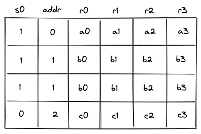
The meaning of columns in the above is as follows:
- Column specifies whether the value in the row should be included into the chiplets bus .
- is a column which starts out at and must either remain the same or be incremented by with every row.
- are contain the roots of the kernel functions. The values in these columns can change only when the value in the column changes. If the column remains the same, the values in the columns must also remain the same.
Constraints
The following constraints are required to enforce correctness of the kernel ROM trace.
For convenience, let's define .
The column must be binary.
The value in the column must either stay the same or increase by .
Finally, if the column stays the same then the kernel procedure root must not change. This can be achieved by enforcing the following constraint against each of the four procedure root columns:
These constraints on should not be applied to the very last row of the kernel ROM's execution trace, since we do not want to enforce a value that would conflict with the first row of a subsequent chiplet (or padding). Therefore we can create a special virtual flag for this constraint using the selector column from the chiplets module that selects for the kernel ROM chiplet.
The modified constraints which should be applied are the following:
Note: these constraints should also be multiplied by chiplets module's selector flag for the kernel ROM chiplet, as is true for all constraints in this chiplet.
Chiplets bus constraints
The chiplets bus is used to keep track of all kernel function calls. To simplify the notation for describing kernel ROM constraints on the chiplets bus, we'll first define variable , which represents how each kernel procedure in the kernel ROM's execution trace is reduced to a single value. Denoting the random values received from the verifier as , etc., this can be achieved as follows.
Where, is the unique operation label of the kernel procedure call operation.
The request side of the constraint for the operation is enforced during program block hashing of the SYSCALL operation.
To provide accessed kernel procedures to the chiplets bus, we must send the kernel procedure to the bus every time it is called, which is indicated by the column.
Thus, when this reduces to , but when it becomes .
Kernel procedure table constraints
Note: Although this table is described independently, it is implemented as part of the chiplets virtual table, which combines all virtual tables required by any of the chiplets into a single master table.
This kernel procedure table keeps track of all unique kernel function roots. The values in this table will be updated only when the value in the idx column changes.
The row value included into is:
The constraint against is:
Thus, when , the above reduces to , but when , the above becomes .
We also need to impose boundary constraints to make sure that running product column implementing the kernel procedure table is equal to when the kernel procedure table begins and to the product of all unique kernel functions when it ends. The last boundary constraint means that the verifier only needs to know which kernel was used, but doesn't need to know which functions were invoked within the kernel. These two constraints are described as part of the chiplets virtual table constraints.
Lookup arguments in Miden VM
Zero knowledge virtual machines frequently make use of lookup arguments to enable performance optimizations. Miden VM uses two types of arguments: multiset checks and a multivariate lookup based on logarithmic derivatives known as LogUp. A brief introduction to multiset checks can be found here. The description of LogUp can be found here.
In Miden VM, lookup arguments are used for two purposes:
- To prove the consistency of intermediate values that must persist between different cycles of the trace without storing the full data in the execution trace (which would require adding more columns to the trace).
- To prove correct interaction between two independent sections of the execution trace, e.g., between the main trace where the result of some operation is required, but would be expensive to compute, and a specialized component which can perform that operation cheaply.
The first is achieved using virtual tables of data, where we add a row at some cycle in the trace and remove it at a later cycle when it is needed again. Instead of maintaining the entire table in the execution trace, multiset checks allow us to prove data consistency of this table using one running product column.
The second is done by reducing each operation to a lookup value and then using a communication bus to provably connect the two sections of the trace. These communication buses can be implemented either via multiset checks or via the LogUp argument.
Virtual tables in Miden VM
Miden VM makes use of 6 virtual tables across 4 components, all of which are implemented via multiset checks:
- Stack:
- Decoder:
- Chiplets:
- Chiplets virtual table, which combines the following two tables into one:
Communication buses in Miden VM
One strategy for improving the efficiency of a zero knowledge virtual machine is to use specialized components for complex operations and have the main circuit “offload” those operations to the corresponding components by specifying inputs and outputs and allowing the proof of execution to be done by the dedicated component instead of by the main circuit.
These specialized components are designed to prove the internal correctness of the execution of the operations they support. However, in isolation they cannot make any guarantees about the source of the input data or the destination of the output data.
In order to prove that the inputs and outputs specified by the main circuit match the inputs and outputs provably executed in the specialized component, some kind of provable communication bus is needed.
This bus is typically implemented as some kind of lookup argument, and in Miden VM in particular we use multiset checks or LogUp.
Miden VM uses 2 communication buses:
- The chiplets bus , which communicates with all of the chiplets (Hash, Bitwise, Memory, and Kernel ROM). It is implemented using multiset checks.
- The range checker bus , which facilitates requests between the stack and memory components and the range checker. It is implemented using LogUp.
Length of auxiliary columns for lookup arguments
The auxiliary columns used for buses and virtual tables are computed by including information from the current row of the main execution trace into the next row of the auxiliary trace column. Thus, in order to ensure that the trace is long enough to give the auxiliary column space for its final value, a padding row may be required at the end of the trace of the component upon which the auxiliary column depends.
This is true when the data in the main trace could go all the way to the end of the trace, such as in the case of the range checker.
Cost of auxiliary columns for lookup arguments
It is important to note that depending on the field in which we operate, an auxiliary column implementing a lookup argument may actually require more than one trace column. This is specifically true for small fields.
Since Miden uses a 64-bit field, each auxiliary column needs to be represented by columns to achieve ~100-bit security and by columns to achieve ~128-bit security.
Multiset checks
A brief introduction to multiset checks can be found here. In Miden VM, multiset checks are used to implement virtual tables and efficient communication buses.
Running product columns
Although the multiset equality check can be thought of as comparing multiset equality between two vectors and , in Miden VM it is implemented as a single running product column in the following way:
- The running product column is initialized to a value at the beginning of the trace. (We typically use .)
- All values of are multiplied into the running product column.
- All values of are divided out of the running product column.
- If and were multiset equal, then the running product column will equal at the end of the trace.
Running product columns are computed using a set of random values , sent to the prover by the verifier after the prover commits to the execution trace of the program.
Virtual tables
Virtual tables can be used to store intermediate data which is computed at one cycle and used at a different cycle. When the data is computed, the row is added to the table, and when it is used later, the row is deleted from the table. Thus, all that needs to be proved is the data consistency between the row that was added and the row that was deleted.
The consistency of a virtual table can be proved with a single trace column , which keeps a running product of rows that were inserted into and deleted from the table. This is done by reducing each row to a single value, multiplying the value into when the row is inserted, and dividing the value out of when the row is removed. Thus, at any step of the computation, will contain a product of all rows currently in the table.
The initial value of is set to 1. Thus, if the table is empty by the time Miden VM finishes executing a program (we added and then removed exactly the same set of rows), the final value of will also be equal to 1. The initial and final values are enforced via boundary constraints.
Computing a virtual table's trace column
To compute a product of rows, we'll first need to reduce each row to a single value. This can be done as follows.
Let be columns in the virtual table, and assume the verifier sends a set of random values , to the prover after the prover commits to the execution trace of the program.
The prover reduces row in the table to a single value as:
Then, when row is added to the table, we'll update the value in the column like so:
Analogously, when row is removed from the table, we'll update the value in column like so:
Virtual tables in Miden VM
Miden VM makes use of 6 virtual tables across 4 components:
- Stack:
- Decoder:
- Chiplets:
- Chiplets virtual table, which combines the following two tables into one:
Communication buses via multiset checks
A bus can be implemented as a single trace column where a request can be sent to a specific component and a corresponding response will be sent back by that component.
The values in this column contain a running product of the communication with the component as follows:
- Each request is “sent” by computing a lookup value from some information that's specific to the specialized component, the operation inputs, and the operation outputs, and then dividing it out of the running product column .
- Each chiplet response is “sent” by computing the same lookup value from the component-specific information, inputs, and outputs, and then multiplying it into the running product column .
Thus, if the requests and responses match, and the bus column is initialized to , then will start and end with the value . This condition is enforced by boundary constraints on column .
Note that the order of the requests and responses does not matter, as long as they are all included in . In fact, requests and responses for the same operation will generally occur at different cycles. Additionally, there could be multiple requests sent in the same cycle, and there could also be a response provided at the same cycle that a request is received.
Communication bus constraints
These constraints can be expressed in a general way with the 2 following requirements:
- The lookup value must be computed using random values , etc. that are provided by the verifier after the prover has committed to the main execution trace.
- The lookup value must include all uniquely identifying information for the component/operation and its inputs and outputs.
Given an example operation with inputs and outputs , the lookup value can be computed as follows:
The constraint for sending this to the bus as a request would be:
The constraint for sending this to the bus as a response would be:
However, these constraints must be combined, since it's possible that requests and responses both occur during the same cycle.
To combine them, let be the request value and let be the response value. These values are both computed the same way as shown above, but the data sources are different, since the input/output values used to compute come from the trace of the component that's "offloading" the computation, while the input/output values used to compute come from the trace of the specialized component.
The final constraint can be expressed as:
Communication buses in Miden VM
In Miden VM, the specialized components are implemented as dedicated segments of the execution trace, which include the 3 chiplets in the Chiplets module (the hash chiplet, bitwise chiplet, and memory chiplet).
Miden VM currently uses multiset checks to implement the chiplets bus , which communicates with all of the chiplets (Hash, Bitwise, and Memory).
LogUp: multivariate lookups with logarithmic derivatives
The description of LogUp can be found here. In MidenVM, LogUp is used to implement efficient communication buses.
Using the LogUp construction instead of a simple multiset check with running products reduces the computational effort for the prover and the verifier. Given two columns and in the main trace where contains duplicates and does not (i.e. is part of the lookup table), LogUp allows us to compute two logarithmic derivatives and check their equality.
In the above:
- is the number of values in , which must be smaller than the size of the field. (The prime field used for Miden VM has modulus , so must be true.)
- is the number of values in , which must be smaller than the size of the field. (, for Miden VM)
- is the multiplicity of , which is expected to match the number of times the value is duplicated in column . It must be smaller than the size of the set of lookup values. ()
- is a random value that is sent to the prover by the verifier after the prover commits to the execution trace of the program.
Thus, instead of needing to compute running products, we are able to assert correct lookups by computing running sums.
Usage in Miden VM
The generalized trace columns and constraints for this construction are as follows, where component is some component in the trace and lookup table contains the values which need to be looked up from and how many times they are looked up (the multiplicity ).
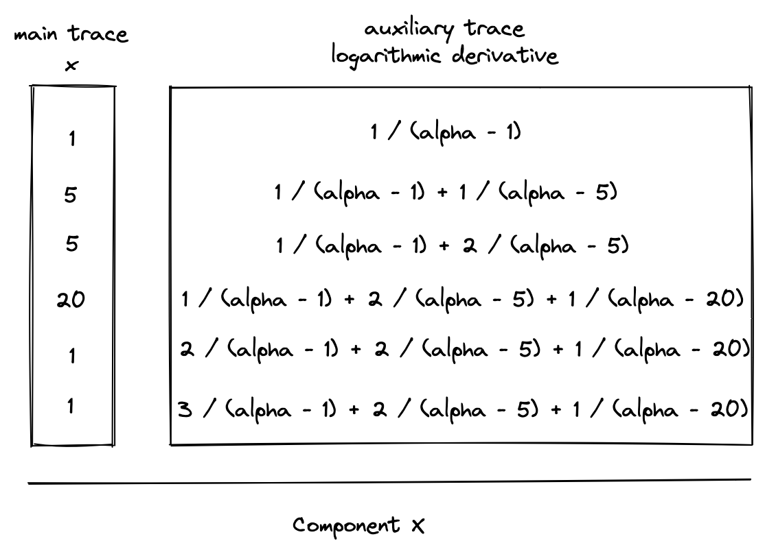
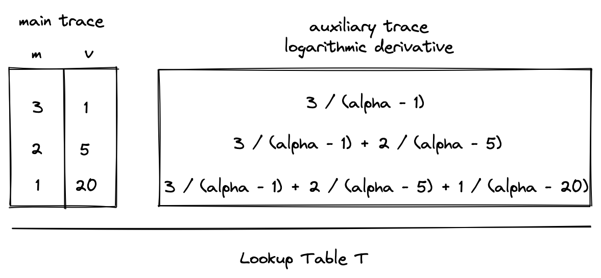
Constraints
The diagrams above show running sum columns for computing the logarithmic derivatives for both and . As an optimization, we can combine these values into a single auxiliary column in the extension field that contains the running sum of values from both logarithmic derivatives. We'll refer to this column as a communication bus , since it communicates the lookup request from the component to the lookup table .
This can be expressed as follows:
Since constraints must be expressed without division, the actual constraint which is enforced will be the following:
In general, we will write constraints within these docs using the previous form, since it's clearer and more readable.
Additionally, boundary constraints must be enforced against to ensure that its initial and final values are . This will enforce that the logarithmic derivatives for and were equal.
Extending the construction to multiple components
The functionality of the bus can easily be extended to receive lookup requests from multiple components. For example, to additionally support requests from column , the bus constraint would be modified to the following:
Since the maximum constraint degree in Miden VM is 9, the lookup table could accommodate requests from at most 7 trace columns in the same trace row via this construction.
Extending the construction with flags
Boolean flags can also be used to determine when requests from various components are sent to the bus. For example, let be 1 when a request should be sent from and 0 otherwise, and let be similarly defined for column . We can use the following constraint to turn requests on or off:
If any of these flags have degree greater than 2 then this will increase the overall degree of the constraint and reduce the number of lookup requests that can be accommodated by the bus per row.
Background Material
Proofs of execution generated by Miden VM are based on STARKs. A STARK is a novel proof-of-computation scheme that allows you to create an efficiently verifiable proof that a computation was executed correctly. The scheme was developed by Eli Ben-Sasson, Michael Riabzev et al. at Technion - Israel Institute of Technology. STARKs do not require an initial trusted setup, and rely on very few cryptographic assumptions.
Here are some resources to learn more about STARKs:
- STARKs paper: Scalable, transparent, and post-quantum secure computational integrity
- STARKs vs. SNARKs: A Cambrian Explosion of Crypto Proofs
Vitalik Buterin's blog series on zk-STARKs:
- STARKs, part 1: Proofs with Polynomials
- STARKs, part 2: Thank Goodness it's FRI-day
- STARKs, part 3: Into the Weeds
Alan Szepieniec's STARK tutorials:
StarkWare's STARK Math blog series:
- STARK Math: The Journey Begins
- Arithmetization I
- Arithmetization II
- Low Degree Testing
- A Framework for Efficient STARKs
StarkWare's STARK tutorial: